Trig for Computer Graphics

Andrew Glassner
https://The Imaginary Institute
25 May 2013

andrew@imaginary-institute.com
https://www.imaginary-institute.com
http://www.glassner.com
@AndrewGlassner

Imaginary Institute Tech Note #2

Table of Contents

• Introduction
• Examples
• The Basic Setup
• Circles: Sine and Cosine
• The Tangent
• Inverses
• atan2
• Solving Our Examples
• Polar Coordinates
• Blending and Easing
• Cyclic Motion

Introduction

A lot of computer graphics involves using geometry to create, position, and move shapes around the screen.

It's often not enough to figure out how things should look for just one picture, because in animated and interactive programs our objects can move, rotate, scale, and otherwise change over time. So we need to figure out where things go on a frame-by-frame basis. For example, we might draw water spraying out of a hose that the user can control. No matter where the hose is moved or pointed, the water should spray out in a nice arc. To draw this, we need to use the current position and orientation of the hose to determine the shape of that arc.

Sometimes we only work with points and lines. Other times we work with angles, or circles. When angles (and circles) enter the picture, the everyday workhorse tools are three little functions (and their inverses) drawn from the general field of trigonometry, or trig for short.

As its name might suggest, trig is the study of triangles. Its a big topic, but here we're just going to focus on a few ideas. These ideas are so useful that they're implemented in just about every graphics library in every programming language on the planet.

It's well worth getting familiar with these trig tools, because they will greatly expand the range of things you can draw and the programs you can create. And as a bonus, they let us create natural-looking motion and blends, and endless repeating patterns of many different kinds. We'll see all of this here.

Examples

To get started, lets look at four example situations where trig tools are useful. Later on we'll see how to use our trig tools to easily solve all of these.

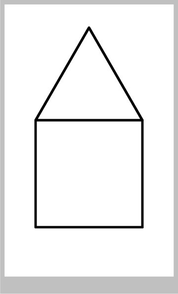
Fitting Shapes Together

In an interactive drawing program, we let someone create squares anywhere. Then they can build a simple house by adding a triangle over the square, as in Figure 1. We want this triangle to be equiangular: that is, all the angles are equal. Given the center and size of the square, what are the coordinates of the tip of the triangle?

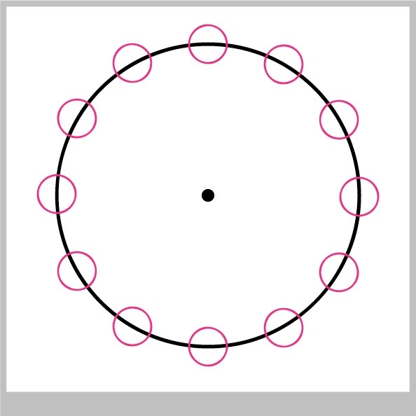
Putting Dots On A Circle

We'd like to let the user place any number of smaller circles evenly around a circle, as in Figure 2. How do we find the centers of those circles?

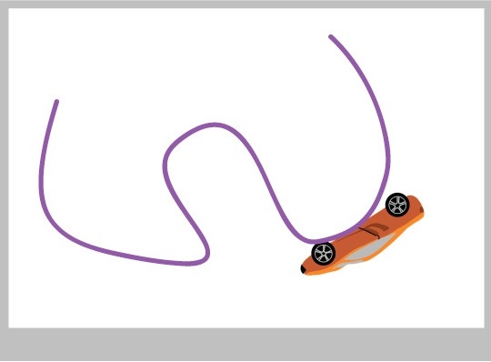
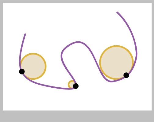
Drawing A Car On A Path

We have a motion path made up of a curve, and a little car that travels on the path, as in Figure 3. At any point on the curve, we can find the line and circle that just "kiss" the curve. We want to rotate the car so it always sits on the curve as it moves. For each point on the curve where the car is located, how much should we rotate the car so it seems to be following the curve?

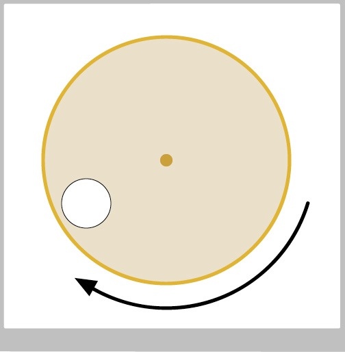
Moving Shapes

In a little game, a big spinning, solid disk has a smaller circle cut out of it, as in Figure 4. The player's goal is to click the mouse in the empty circle as it moves. To see if they managed it, we need to test if their mouse click point is inside the circle, so we need the circle's center at that moment. How do we find the center of that empty circle as it rotates?

The Basic Setup

We're going to talk a lot about coordinates and angles here, so let's agree on our measuring conventions.

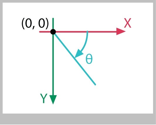
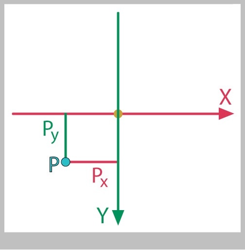
I'll say that the positive X axis goes to the right. In most geometry books, the Y axis goes up. But in many computer graphics libraries (such as the one built into Processing), the Y axis goes down, so I'll use that convention here. I'll measure angles starting at 3 o'clock (that is, the positive X axis) and say that positive angles go clockwise.

Figure 5 shows the setup.

To keep things simple, I'll refer to all of our angles using degrees. Keep in mind that almost every math library in the world uses radians instead. I cover degrees, radians, and how to go back and forth, in the videos "Angles" (Week 4, Group 2, Video 5) and "Degrees And Radians" (Week 4, Group 2, Video 6).

Circles: Sine and Cosine

Circles are super-useful pieces of geometry. A key step in doing all kinds of geometry is to to find the x and y coordinates of a point on a circle. Let's look at how to get those.

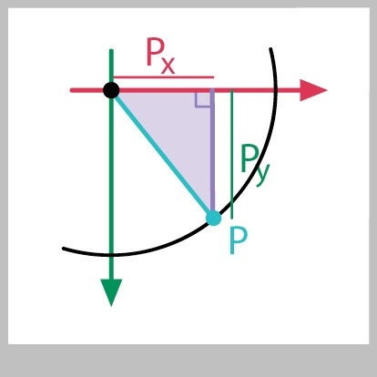
Figure 6 shows a circle of radius 1, centered at the origin, or the point (0, 0). To keep the diagrams simple, all of my circles will be centered at the origin unless I explicitly say otherwise. If you want to move a circle so that it's centered at some other point, say $(cx, cy)$, you need only add $cx$ and $cy$ to every point.

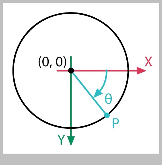
On the circle in Figure 6 I've marked a point that I've named P. I've also drawn a line from the circle's center to P, and marked the angle between this line and the X axis. Following convention, I've named this angle with a lower-case Greek letter; in this case, it's theta, written with the Greek letter $\theta$.

Let's suppose that we know the angle $\theta$, and we want to find the x and y values of point P. This comes up so often that people have made it super-easy.

Conceptually, you can imagine that someone sat down with pencil and paper, drew a circle of radius 1, drew an angle of $\theta$, and put a dot at P. Then they got out their ruler and measured the $x$ and $y$ values of P, which I'll write as $P_x$ and $P_y$. Then they did this again and again, for one angle after another. When they were done, they had a huge table of x and y values. Then nobody would have to repeat their work any more. To find the x and y values of a point at any value of $\theta$, you would just look at the row for $\theta$ in the table. If your radius wasn't 1, you'd just multiply those values by the radius you had.

People may actually have done that at one point, but now we have little functions to compute those values, and they're in every programming language's math library. You can hand one of these functions your value of $\theta$, and you get back the x value of the point at that angle, on a circle of radius 1. Hand your $\theta$ to another function, and you get back the y value.

The names of these functions come from their origins in trigonometry. The x value comes from the cosine function, and the y value comes from sine . In your math library, these are almost certainly abbreviated as cos() and sin(). You hand them a single float that holds your angle $\theta$ (expressed in radians), and you get back the x value from cos(theta) , and the y value from sin(theta) (of course, you can name your angle anything you like, but theta is a common convention). Here's how you'd write it.

// Find the point at angle theta for a circle of radius 1 centered at (0, 0)
float x = cos(theta);
float y = sin(theta);

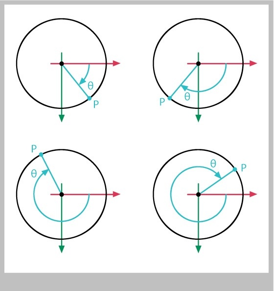
This all works no matter where your point P is located - that is, no matter what value of you hand to sine and cosine. Any value works fine - if its outside the range 0-360 (or 0-$2\pi$), your point just wraps around the circle over and over.

But wait a second, the x and y values we're getting are for a circle of radius 1. What if the circle has some other radius, like 1/2 or 3?

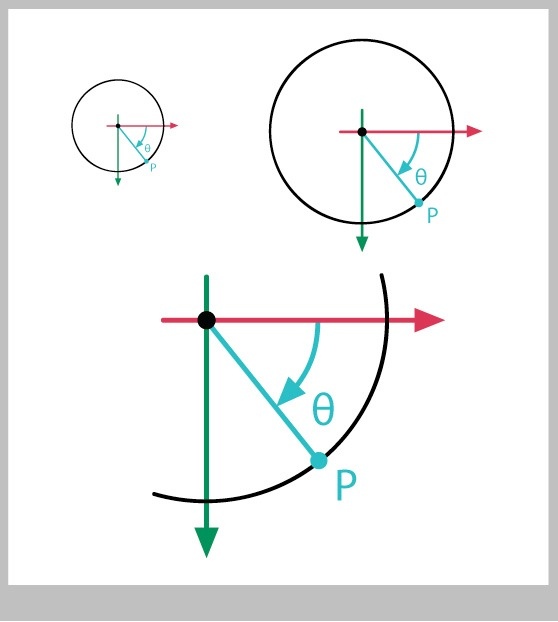
The answer, happily, is that you simply multiply the x and y values by the radius of the circle. In Figure 8, we see a couple of circles with radii 1/2 and 3. For any angle $\theta, youd just multiply the values from sine and cosine by 1/2 and 3. In fact, for any radius r,

// Find the point at angle theta for a circle of radius r centered at (0, 0)
float x = r * cos(theta);
float y = r * sin(theta);

As I mentioned earlier, if the circle isn't centered at (0, 0) we only need to add its center values to our x and y:

// Find the point at angle theta for a circle of radius r centered at (Px, Py)
float x = Px + (r * cos(theta));
float y = Py + (r * sin(theta));

So far weve talked about circles. Where are the triangles I talked about before?

They're already there! We can draw a little right triangle in our circle. The legs are parallel to the X and Y axes, and the hypotenuse is the radius, as in Figure 9.

This diagram is a great thing, because it means that we can find not only the x and y values for points on a circle, but we can find the lengths of the legs of any right triangle, whether its part of a circle or not, if we know one other angle and the length of the hypotenuse. Figure 10 shows the idea.

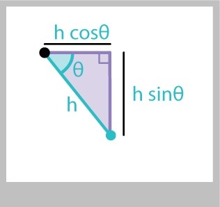
The lengths of the legs are just the same as before (I'll name the hypotenuse $h$):

x = h * cos(theta);
y = h * sin(theta);

Notice that if know and the x value, the first of these expressions can give us the length of the hypotenuse. Similarly, if we know and y, we can find the hypotenuse from the second expression:

// both h1 and h2 will have the same value
h1 = x / cos(theta);
h2 = y / sin(theta);

Finally, we can go back to the previous pair and divide both sides by $h$. That lets us find values for the cosine and sine without ever calling sin() or cos(). This doesn't come up often, but sometimes its useful to find the sine or cosine of an angle even when you don't know the angle itself. If we just divide both sides of the first pair of relations by $h$, we get those values:

float cosTheta = x / h;
float sinTheta = y / h;

Both sine and cosine can become 0, and sometimes $h$ can be 0, so if you're going to divide like this in your program you'll want to check to make sure you're not dividing by zero. But what if you are dividing by zero? What should your result be? Trying to handle this is a really robust way is a mess. Luckily, we rarely need to do this division, since there's a different function that we'll almost always use instead. We'll get to that in a moment, after we cover some background.

The Tangent

There's a third function that is just as useful as sine and cosine. Called tangent, it too is a function of your input angle. It returns the ratio of the sine to the cosine. In your graphics library, this is almost surely called tan(). All three of these lines produce the same value:

// these all produce the same value (assuming you're not dividing by zero!) float t1 = tan(theta); float t2 = sin(theta) / cos(theta); float t3 = y / x;

What good is this new function? The beauty is that we can find the length of a triangle's leg even without knowing the length of the hypotenuse. If we know the angle $\theta$, and the length of either of the two legs next to the right angle, we can use tangent to find the other leg:

y = x * tan(theta);
x = y / tan(theta);

If the angle isn't adjacent to the X axis, then we might need to re-label these relationships. This can get confusing. So instead, we usually refer to the adjacent side (the leg next to the angle we know) and the opposite side (the leg opposite the angle we know), as in Figure 11.

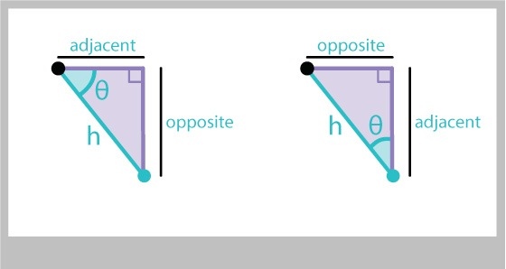
Now if we know the lengths of these legs, we can find the tangent with ever calling tan(), just as we did for sine and cosine:

float tanTheta = opp / adj;

More commonly, we use tan() to find either leg, from one angle and the other leg:

float opp = adj * tan(theta);
float adj = opp / tan(theta);

Youll sometimes see sine and cosine defined in terms of the adjacent and opposite legs. If you have a right triangle and you know the length of the hypotenuse and one of the angles (other than the right angle), you can find the length of the leg that's adjacent to, or opposite from, the angle you know. Here's sine and cosine, followed by tangent (which we just saw), expressed in terms of the opposite and adjacent lengths:

$$ \sin(\theta) = \mbox{opp} \;/\; \mbox{hyp} \\ \cos(\theta) = \mbox{adj} \;/\; \mbox{hyp} \\ \tan(\theta) = \mbox{opp} \;/\; \mbox{adj} $$

Countless people around the world remember these with the little made-up word sohcahtoa (rhymes with "mocha boa"). The first three letters, soh, are to remind you that Sine is Opposite over Adjacent, then cah is for Cosine is Adjacent over Hypotenuse, and toa is for Tangent is Opposite over Adjacent. It probably sounds ridiculous, and it is, but if you can get that word in your memory you'll find it's a lot easier than memorizing the three relationships. And you'll know a secret word shared by programmers and mathematicians all over the world!

Using the labels opp and adj is better than using x and y, because that lets us draw the triangle any way we like, without worrying about whether the legs are even lined up with the X and Y axes.

Inverses

You can run each of these three trig functions "backwards." For example, if you know a value of $\sin(\theta)$, you can get the value of $\theta$ that produced it.

Each of sine, cosine, and tangent has a corresponding "backwards" function that lets you find the input that produced a particular output. These are often called "inverse functions," but math libraries almost always call them "arc functions." So the inverse functions are arc-sine, arc-cosine, and arc-tangent. By universal convention, the routines in your math library just use the letter a rather than the whole word arc. Thus you'll find asin(), acos(), and atan() in your library. They each take as input a floating-point number, and they return the value of $\theta$ (as always, in radians) that would have produced that output for that function.

For example, let's find the sine of 90 degrees ($\pi$/2 radians), and then run that back through asin():

float theta = 3.1415926535/2.0;  // PI/2
float sinTheta = sin(theta);
theta2 = asin(sinTheta);

If you run a program like this, you'll find that theta2 has about the same value as theta (in a perfect world they'd be exact, but in the real world of finite-precision computers, they'll probably be different by a very, very tiny amount).

Frankly, you probably won't use sine, cosine, and tangent very much. They definitely come up and they have their uses, but they're not the workhorses of trig and geometry in programs. That honor goes to a fourth function that belongs to the family, and that's the one you'll use most of the time.

It's just the atan() function we saw before, but in a slightly different form. Here's why we need this.

Suppose you're drawing some stuff on the screen, and the location of a point P is given by the triangle in Figure 12, where for simplicity we'll say that the legs are parallel to the X and Y axes.

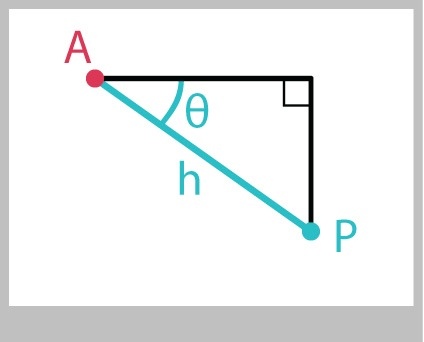
If you know the point A, the distance from A to P (that is, the length of the hypotenuse), and the angle $\theta$, it's easy to find the location of P. Let's call its values Px and Py.

Px = Ax + (h * cos(theta));
Py = Ay + (h * sin(theta));

Now let's suppose that we already know the x and y values, and we want $\theta$. This actually comes up very frequently. For example, the location of point P might be controlled by the user's mouse, so we get back the mouse coordinates in x and y from the computer. Thus we have x and y, but we want to rotate something around by the corresponding $\theta$. How can we find $\theta$?

No problem, we can just use one of the inverse functions. Let's pick arc-tangent, or atan(). Then we can write the two legs of the triangle as the distances of the mouse to the circle center at A, and use atan() to get the angle:

float theta = atan((Py-Ay) / (Px-Ax));

This works just fine for the triangle in the figure, but notice that the user could put the point P directly under A, so it has the same x value as A, but a larger y value. Then Px-Ax would be zero. And you probably know that dividing by zero can cause your program to crash, or at least just go haywire. You really need to avoid dividing by zero, ever.

So you could put in a test to see if the difference in X is zero, and if so, you'll just stick the correct value into theta without calling atan():

float theta = 0;   // give it a starting value
if ((Px-Ax) == 0) {
	theta = PI/2;  // that's 90 degrees
} else {
	theta = atan((Py-Ay) / (Px-Ax));
}

That's better, but nobody wants to have to do that every time in every program. And if Px-Ax is very, very small (or very, very big) then the finite precision of real-world computers means that the result could be less accurate than you'd like.

There's an even bigger problem. Suppose the mouse is located above point A - that is, it has the same x value, but smaller y value. The difference in x values is still 0, but the angle here should be 270 degrees, not 90. This is just the tip of an iceberg of problems.

Simply said, atan() just can't do its entire job properly with just the one number it takes as input. But if it had both the x and y values separately, it could test them for various relationships, and then produce the correct angle in response.

atan2

Happily, there's no need to mess around with atan() and issues of dividing by zero. The work's been done for you. Just call the two-argument form of atan(), almost always called atan2(). Because in atan() you create the argument using the y value divided by the x value, in atan2() you almost always follow the same order: first name the y value, and then the x.

So to use atan2(), you don't hand the result of y/x to the function, but instead, you hand it each of these values in turn:

float theta = atan2(Py-Ay, Px-Ax);

This will return the correct value for all points A and P, no matter how they're oriented with respect to one another.

The function atan2() takes care of all the details that go into getting the right answer. It's almost always the way to go when you need to find an angle from a triangle's legs. Its a very rare day when you find yourself needing the one-argument atan() rather than the much superior two-argument version atan2().

Although you can easily imagine corresponding two-argument forms of sine and cosine, they turn out to be tricky to use in practice. So the only two-argument inverse (or arc) function that you'll usually in your library see is atan2(), and it's extremely rare to ever really need the others.

The most important thing to keep in mind when using atan2() is that the arguments are in the order y, then x. Just about every other graphics function in the world takes its arguments in the order x, then y, so keep in mind that atan2() is the one weird exception to this convention.

Unfortunately, there are a few libraries in the world that define their version of atan2 to take x first and then y. I don't know why they do this; maybe they like having everything be x first, then y. But since almost everyone everywhere knows that atan2 goes the other way, they're definitely defying the standard convention (which of course is itself defying convention). In any case, check your documentation for the right order of x and y for the language or library you're using.

Solving Our Examples

We now have everything we need to program up our four sample problems. Let's re-visit them.

Fitting Shapes Together

In an interactive drawing program, we let someone create squares anywhere. Then they can build a simple house over the square, as in Figure 13. We want the triangle on top of the house to be equiangular: that is, all the angles are equal. Given the center and size of the square, what are the coordinates of the tip of the triangle?

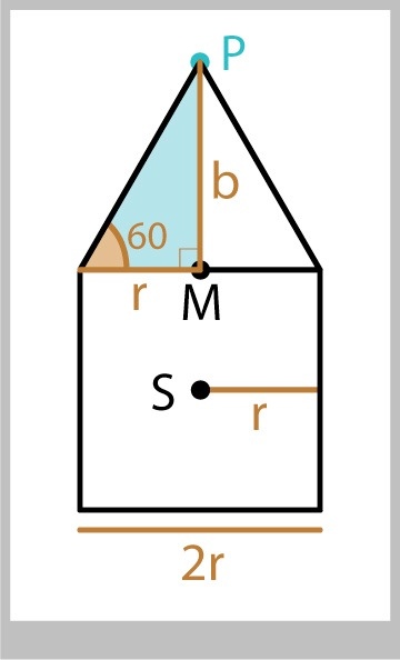
Let's label the square as having a center point S, and a "radius" $r$, which is the distance from S to the middle of any side. Next, let's split the triangle into two right triangles.

Look at the blue triangle. The bottom leg is merely $r$. The angle in the bottom-left is 60 degrees, because all three angles of the triangle are the same (and must add up to 180 degrees). So we know one side and an angle. To find the vertical height of the triangle, which I've labeled $b$, we can use tangent. The leg opposite our 60-degree angle is $b$, and the leg adjacent is $r$. So, because $\tan(\theta) = \mbox{opp}\;/\;\mbox{adj}$, we have

$$ \tan(60) = b/r $$

We can multiply both sides by $r$ to find the height of the triangle, $b$:

b = r*tan(radians(60));

where I used radians() to convert 60 degrees to radians. The point M in the middle of the top of the square is at (Sx, Sy-r). The point P is $b$ units above that:

Px = Sx;
Py = (Sy-r)-b; 

We could roll the expression for b into this last line as

Py = (Sy-r) - (r*tan(radians(60)));

And we're done. We have expressions for Px and Py, so we know where point P is.

Putting Dots On A Circle

We'd like to let the user place any number of smaller circles evenly around a circle, as in Figure 14. How do we find the centers of those circles?

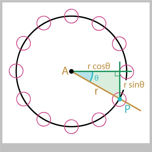
Let's say the big circle is centered at A, and it has a radius of r. We want to place N little circles around this circle. Since the circle has 360 degrees, we only need to rotate by 360/N to find the first, 2*(360/N) to find the second, and so on:

angleStep = 360.0/numCircles;
for (int i=0; i<numCircles; i++) {
	theta = i * angleStep;
	Px = Ax + (r * cos(radians(theta)));
	Py = Ay + (r * sin(radians(theta)));
	// draw new little circle at (Px, Py)
}

where I again used the function radians() to convert our angle in degrees into an angle in radians.

Drawing A Car On A Path

We have a motion path made up of a curve, and a little car that travels on the path, as in Figure 15. At any point on the curve, we can find the line and circle that just "kiss" the curve. We want to rotate the car so it always sits on the curve as it moves. For each point on the curve where the car is located, how much should we rotate the car so it seems to be following the curve?

Before we dig in, let's agree on how to orient the car. I'll say that the default drawing for the car has it facing down, with its roof to the right, as in Figure 16.

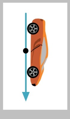
Positioning the car on the curve is easy: just add the curve points x and y values to the car values. Let's see how much we need to rotate the car around its origin (the black dot in Figure 16) so it seems to be following the curve.

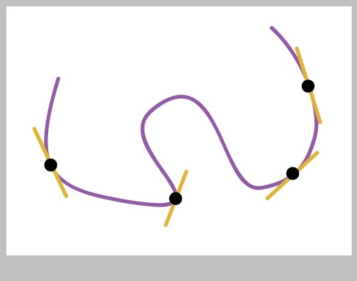
I'll start by drawing a picture of the "kissing" lines mentioned in the problem statement. The kissing line is usually called the tangent line , and it's the line that goes through a given point on the curve but only touches the curve at that one spot (in the neighborhood around the point, anyway). The word tangent here is conceptually related to our previous use of the word tangent for a specific trig function, but it's probably best to think of this as one word used with two different meanings. We can ask the computer for the tangent line for any point on the curve. When we give the computer P, we usually get back another point on the line (and not just P again!).

Figure 17 shows a few examples of the tangent lines at different points on a curve.

We can also ask for a circle, called an "osculating circle" (from ovulum , Latin for "kissing"). This is the circle that best hugs the curve at a given point. We'll usually get back the circle's center and radius.

Figure 18 shows a few examples of the circles for different points on a curve.

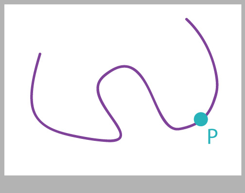
Now we're set. Suppose we want to draw the car at point P in Figure 19.

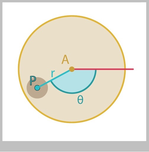
We ask for the osculating circle at P, and we get back a circle with center C and radius r, as in Figure 20.

The only thing we need to know now is the angle $\theta$. Since we know both P and C, we can find the lengths of the two legs as Py-Cy and Px-Cx. Since we want to find the angle, we have a job for atan2():

theta = atan2(Py-Cy, Px-Cx);

Now we have everything we need. First, move the car to P. Second, rotate by $\theta$. Third, draw the car.

Here's the code:

// osculating circle for point P has center C and radius r
theta = atan2(Py-Cy, Px-Cy);  // find the angle
translate(Px, Py);            // move origin to point P
rotate(theta);                // rotate to match curve
drawCar();                    // draw the car

Moving Shapes

In a little game, a big spinning, solid disk has a smaller circle cut out of it, as in Figure 21. The player's goal is to click the mouse in the empty circle as it passes by. To see if they managed it, we need to test if their mouse click point is inside the circle, so we need the circle's center at that moment. How do we find the center of that empty circle as it rotates?

Let's say that the wheel is spinning by d degrees every frame, starting at 0 degrees on frame 0. Then on frame f it has rotated by d*f degrees. If this number grows past 360, it's no problem: all the trig functions will happily work with numbers of any size (and even negative ones!).

Let's label the point at the center of the big circle A, and the center of the little cut-out as P. The point P starts on the X axis, r units to the right of A. So at any given frame,

theta = frameNumber * radiansPerFrame;
Px = Ax + (r * cos(theta));
Py = Ay + (r * sin(theta));

Now we can check the mouse's x and y values with respect to the circle centered at (Px, Py).

Polar Coordinates

Polar coordinates give us a different way to write down the location of a point in the plane. This alternate description is sometimes exactly what you want to describe where your objects are located.

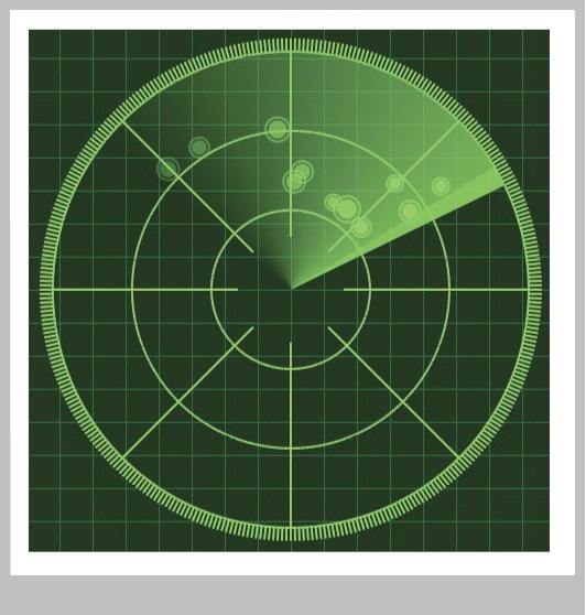
For example, if you've ever seen a picture of an old-fashioned radar screen, like in Figure 22, you've seen this system in action. The person tracking an incoming object on this screen doesn't care about the x and y values of a blip. Instead, the operator wants to know "What direction is it coming from?" and "How far is it?"

Before we look at this, lets revisit the coordinate system weve been using all along: the familiar X and Y axes. Knowing the point at the origin of the system, and the orientation of the axes, then you only need 2 numbers, x and y, to uniquely and completely identify any point on the plane.

Figure 23 shows this system along with a point P. This X and Y system is often called the Cartesian coordinate system (after mathematician Ren Descartes), and the numbers x and y that identify a point in the form (x,y) are called Cartesian coordinates.

We can also think of a system like the radar system: a series of concentric circles and lines radiating outward from an origin. To identify the location of a point P, we can use two numbers: the angle by which to rotate (clockwise from 3 o'clock), and the distance by which to move along this direction. Conventionally, the angle is called $\theta$ and the distance is $r$, and they are shown in Figure 24.

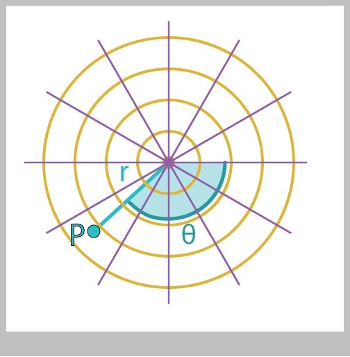
The $r$ and $\theta$ system is called the polar coordinate system , and numbers r and that identify a point in the order $(r, \theta)$ are called polar coordinates.

We use the Cartesian system most of the time in graphics, but when the polar system is appropriate, it is worlds easier to use. We used polar coordinates to solve our fourth example problem above, though we didn't name them at the time.

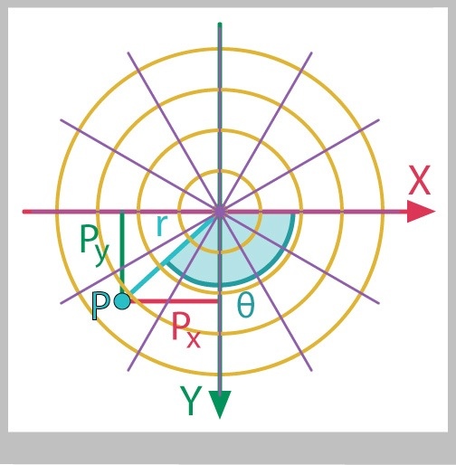
To get back and forth between either system is easy if we use our trig routines. To show how the coordinates are related, Figure 25 show the point P on both sets of coordinates simultaneously. The point $(P_x, P_y)$ is also the point $(r, \theta)$.

In code, we can convert from polar to Cartesian coordinates this way:

// convert from (r,theta) to (x,y)
x = r * cos(theta);
y = r * sin(theta);

and we can just as easily convert from Cartesian to polar, using our new friend atan2():

// convert from (x,y) to (r,theta);
r = sqrt((x*x)+(y*y));
theta = atan2(y, x);

Blending and Easing

Sine and cosine have another great trick up their sleeves that has nothing obvious to do with triangles or even circles.

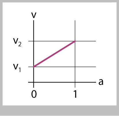
This trick comes from the way we often move and blend things. Many systems provide a function called lerp() (for "linear interpolation"), which blends two floating-point numbers:

float v1 = 3;
float v2 = 5;
float a = .7;
float v = lerp(v1, v2, a);

The blend starts with value v1 when a=0, and ends with value v2 when a=1 Figure 26 show the output v given the inputs v1, v2, and a.

Is this useful in practice? All the time.

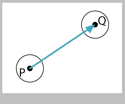
Suppose that we're drawing a ball that moves across the screen. Initially, it's sitting at point P with coordinates (Px, Py). It then starts moving at time t0, and stops moving at time t1, stopping at point Q, or (Qx, Qy), as shown in Figure 27 ( t0 and t1 could be frame numbers, or seconds elapsed since the program started running).

How would we program this movement from P to Q? Let's use a as the variable that controls the blending (we called it v above). We could use Processing's built-in map() to give us a value of a that starts at 0 at t0 , and goes to 1 at t1 . Then we can use r to blend, or lerp, the x and y values:

float t0 = frameCount/100.0;          // some measure of time from 0 to 1
float a = map(timeNow, t0, t1, 0, 1); // a is 0 when timeNow=t0, 1 at t1
float xNow = lerp(Px, Qx, a);         // blend x values
float yNow = lerp(Py, Qy, a);         // blend y values
drawBallCenteredAt(xNow, yNow);       // draw ball at this location

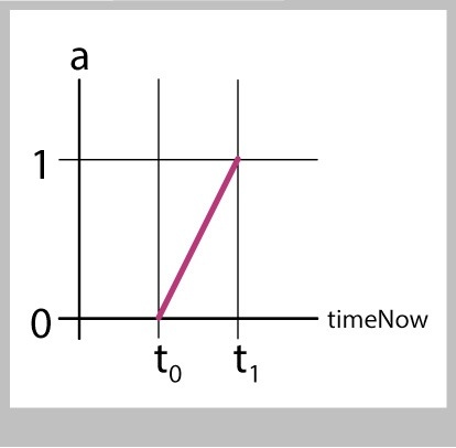
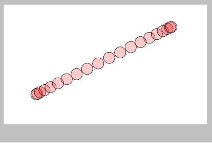
As time goes up, the value of a will increase smoothly and at a fixed pace, as in Figure 28.

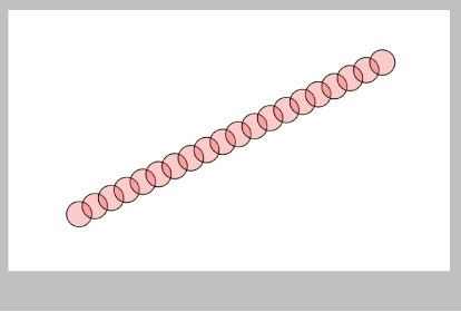
This means the ball will also move from P to Q smoothly and at a fixed pace, as in Figure 29.

So far so good. Our code above isn't checking to make sure that timeNow is really between t0 and t1 , so we add some code to check for that. If the time is before t1 , we know we're sitting at point P, and after t2 , we know we're at Q.

if (timeNow < t0) {         // when timeNow < t0, we're at P
   xNow = Px;
   yNow = Py;
} else if (timeNow > t1) { // when timeNow > t1, we're at Q
   xNow = Qx;
   yNow = Qy;
} else {
   a = map(timeNow, t0, t1, 0, 1); // in between values mean blend
   xNow = lerp(Px, Qx, a);
   yNow = lerp(Py, Qy, a);
}
drawBallCenteredAt(xNow, yNow);

Note that we could get the same result by testing the value of a instead of timeNow . This code produces the same results as the code above:

a = map(timeNow, t0, t1, 0, 1);
if (a < 0) {
   xNow = Px;
   yNow = Py;
} else if (a > 1) {
   xNow = Qx;
   yNow = Qy;
} else {
   xNow = lerp(Px, Qx, a);
   yNow = lerp(Py, Qy, a);
}
drawBallCenteredAt(xNow, yNow);

An even shorter way to write this second version is to clamp the value of a between the values 0 and 1. This code produces the same results as the two preceding examples (there's a built-in Processing routine called constrain() that we could use for this job, but I'll write the two tests out explicitly so they're clear):

a = map(timeNow, t0, t1, 0, 1);  
if (a < 0) a = 0;
if (a > 1) a = 1;
xNow = lerp(Px, Qx, a);
yNow = lerp(Py, Qy, a);
drawBallCenteredAt(xNow, yNow);

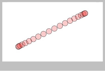
What kind of motion would this produce? Before t0 , the ball is just sitting at point P. Then at time t0 , it suddenly lurches into motion, traveling at constant speed towards point Q. Once it reaches Q, at time t1 , it abruptly slams to a full stop, and then just sits at Q from then on.

This kind of sudden start and stop will almost always catch a viewer's eye, and it will feel somehow "wrong to almost everyone. Nothing in the real world moves in this way, bursting instantly from a full stop to constant speed and then instantly stopping again. Even if they can't tell you why, your audience will know that something doesn't "feel right" in this animation.

Real objects, of course, slowly gain speed at the start of their motion, and gradually come to a stop at the end. Even if these acceleration and deceleration intervals are short, they're there. And right now they're missing. Let's fix that by changing how we compute the value of the variable a , which is controlling our blending.

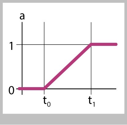
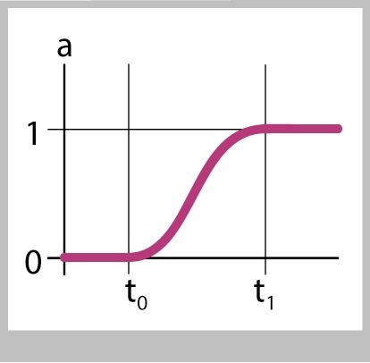
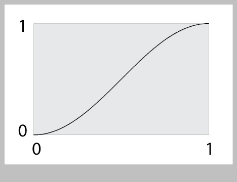
Figure 30 shows a plot of what we have now. We can see that the value of a is 0 before t0 , then it abruptly starts growing, then at time t1 it instantly stops. When we use a to blend the x and y values of P and Q, they have the same general form: they have a value, they instantly start to change at a constant speed, and then instantly stop. Those sudden starts and stops correspond to the sharp corners in the plot. If we could smooth out those corners, then wed smooth out the resulting motion.

Suppose that we changed the way we created a , so that it slowly changes at the start and slowly comes to a halt at the end, as in Figure 31. The value of a is still 0 at t0 and it's still 1 at t1, but it starts and slows gracefully rather than abruptly.

Then the motion of the ball would follow this smooth change, and we'd get results like Figure 32.

When we see the ball move like this, it looks much, much better. Animators call this kind of smooth curve a blending curve, or an easing curve , and they use it to make objects seem to ease in to motion at the start, and ease out at the end.

We could implement this with a little function called ease() that takes our original value of a as input, and returns a new value that starts and ends gracefully.

If we have this function, then we only need one new line of code, which we can place after the line that clamps a from being larger than 1:

if (a > 1) a = 1;
a = ease(a);   // reshape a for smoother changes

This is almost always a good idea. The resulting motion doesn't call attention to itself with sudden jerks at the start and end, and the acceleration and deceleration just "feel" like all the real objects we've seen in the real world for our entire lives.

Here's the reason were discussing all of this now: it turns out that if we plot the values of the sine and cosine curves, they contain a shape pretty close to the easing curve we just drew. These curves don't actually match the real physics of most objects, but it just so happens that they're close enough that they almost always look great.

So let's look at these curves and then see how to use them to write the ease() function we just used.

Figure 33 plots the sine, cosine, and tangent curves from 0 to 360 degrees. Outside of that range, they simply repeat over and over.

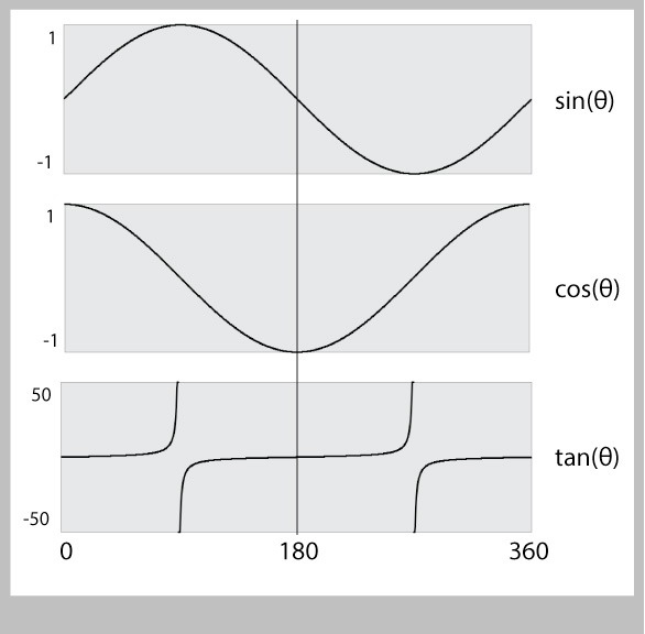
Let's look first at the tangent: it goes crazy at 90 and 270 degrees, flying off to infinity (that's one of the things that atan2() saves us from having to worry about). So I'm going to cross tangent off our list of possible blending functions.

You can see that sine and cosine look very similar. In fact, they are exact copies of one another, except that they are shifted by 90 degrees with respect to each other. Since we're only interested in the shape of the curves right now, we can pick either one. There's no rule, but I usually use cosine for blending, so let's use that.

My plan will be to take the first half of the cosine curve, and re-shape it to look like an easing curve. That is, I'll use the cosine curve to help us write the function ease() above.

I've drawn just the first half of the cosine curve (from 0 to 180 degrees) in Figure 34.

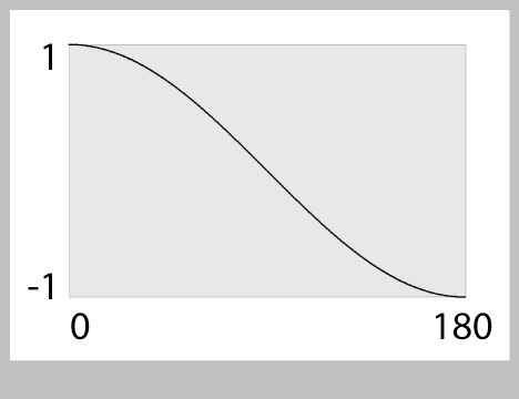
You can see that the input runs from 0 to 180, and the output runs from 1 to -1. We want to make it so the input runs from 0 to 1 (since that's what we're computing for a above), and we get an output from 0 to 1. So step 1 is to take our input value from 0 to 1 and multiply it by 180:

float ease(a) {
   float angle = a*180;
   // ...
}

Great, so now we can hand ease() a value from 0 to 1, and weve built an angle from 0 to 180 to hand to cosine. So lets do that:

float ease(a) {
   float angle = a*180;
   float cosVal = cos(radians(angle));
   // ...
}

where here I've used radians() to convert our angle from degrees to radians. You could skip this if you multiplied the input by $\pi$ (about 3.14) rather than 180. This is, in fact, a little faster, and how most people do it:

float ease(a) {
   float cosVal = cos(a * PI);
   // ...
}

Our variable cosVal runs from -1 to 1, but we want output values from 0 to 1. There are lots of ways to do this, but the easiest one is to let the computer do all the work. Let's hand this value to map() , and tell it to convert values in the range (-1, 1) to new values in the range (0,1):

float ease(a) {
   float cosVal = cos(a * PI);
   cosVal = map(cosVal, -1, 1, 0, 1);
   // ...
}

Oh, we're close, but we're upside-down. We want the curve to have the value 0 at the start, and 1 at the end. The easiest way to do this is to just flip the range that map() is using for the output, from (0,1) to (1,0):

float ease(a) {
   float cosVal = cos(a * PI);
   cosVal = map(cosVal, -1, 1, 1, 0);
   return (cosVal);
}

That does it. We return cosVal and we're done.

Plotting this gives us Figure 35. We feed it values from 0 to 1, and we get back new values from 0 to 1, only theyve been smoothed.

The code for ease() above is just fine. But if we want to make our program shorter, we can combine some of these lines. Merging the first two gives us:

float ease(a) {
   float cosVal = map(cos(a * PI), -1, 1, 1, 0);
   return (cosVal);
}

and of course we could just return this value immediately:

float ease(a) {
   return map(cos(a * PI), -1, 1, 1, 0);
}

There's nothing wrong with this final version, but there's nothing wrong with any of the longer ones above, either, and they're easier to read. Use whatever works best for you.

When we use this ease() function to move the ball, we get Figure 36.

In motion, that looks pretty darned great: the ball picks up speed, moves, then slows down to a halt. This ease() function definitely does the job we wanted.

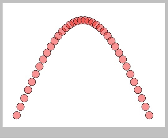
We can do the same thing for any motion. Figure 37 shows a ball on a curved path, perhaps while bouncing along the ground. Here the ball slows down near the top of its arc, like a real ball. I used the first half of the sine function to find the y value for the ball as it moved to the right, so the shape looks just like the sine curve.

This easing technique isn't just for motion. It makes almost any kind of transition look better. If you're blending colors, for example, try easing in and out of the blend. Or if you're showing how one shape deforms into another, try easing in and out of the shape changes. Generally speaking, any time you find yourself blending one thing to another, no matter what the things blended are, no matter if that blend is visible on a single image or changes over time, try using an ease function and see if that makes it look better. More times than not, it will.

People have developed more complicated easing curves that give you control over how fast they get going and how they slow down at the end. Though those blending curves are usually slower to compute and more complicated to program, in some applications its nice to have that extra control so you can shape your blend in just the way you like.

But using a piece of the cosine curve for easing is a time-honored trick that has been used by untold animators for decades, and now it's in your toolbox, too.

Cyclic Motion

But wait, there's more!

Let's draw a picture of the sine wave from some big negative value of up to some big positive value, as in Figure 38.

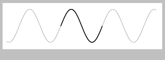
It's beautifully smooth when it repeats. As the value of $\theta$ goes from 0 to 360 degrees (or 0 to $2\pi$ radians), we say that it covers, or passes through, one full cycle. As $\theta$ continues growing, the cycle repeats, over and over, but we never see a break or jump.

This make sine (and cosine) perfect for repeating motion. We already know that we can use sine and cosine to move a point around a circle, just by cranking up the angle forever. But we can use these functions for lots of other kinds of motion, too.

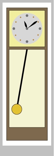
A classic example is the pendulum on a grandfathers clock, as in Figure 39.

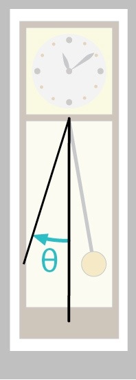
Let's say that each frame is drawn at a time given by the variable time (this might be expressed in seconds or frames). Let's use time to find the angle of the pendulum at each frame. I'll measure the angle as a positive or negative amount relative to straight down, as in figure 40.

Just for variety, I'll choose to use sine. I'll hand the value of time to sin(), and get back a number from -1 to 1. Then I'll scale that by the range of angles that I want for the pendulum. To give myself more control, I'll multiply the time by a value that I'll call speed. That will let me control how fast the pendulum swings:

pendulumAngle = angleRange * sin(time * speed);

That's all there is to it! Now we just use our normal tools to rotate by this angle before we draw the pendulum. We can manually tweak speed up and down until the pendulum swings the way we like.

Note that sine is returning values from -1 to 1, which is just what we want to swing our pendulum from a negative value of $\theta$ to a positive one and back again, over and over.

To control this with a little more finesse, remember that it takes 360 degrees for the sine wave to repeat once. Let's suppose that our variable time is the current number of seconds since the program started, and that we want the pendulum to complete one full left-to-right-to-left swing each second. Then we could multiply time by 360, and the pendulum would complete one full swing exactly once per second:

pendulumAngle = angleRange * sin(radians(time * 360));

Here I used radians() to convert our angle in degrees to radians, which is what sin() expects (if we instead multiplied by $2\pi$, or about 6.28, then our angle would be in radians and we could skip this step, as in the development of ease() above). If we still wanted to be able to hand-tune the time it took for the pendulum to swing, we could still multiply by speed:

pendulumAngle = angleRange * sin(radians(time * 360 * speed));

Now speed has a very physical interpretation: its how many times the pendulum completes one full swing per second. Values of speed below 1 will slow the pendulum down, and values larger than 1 will speed it up.

We can let this program run forever, and the pendulum will smoothly swing back and forth. It will even slow down at the left and right ends of each arc, and speed up at the bottom, easing into and out of its swing just like a real pendulum. All thanks to sine!

You can use this technique for any kind of repeating, or cyclic motion.

Once you start using sine and cosine for easing and motion, you'll find yourself using them all the time!

Thanks to Steven Drucker for helpful advice that greatly improved this document.