The AU Library:
Waves
Andrew Glassnerhttps://The Imaginary Institute
15 October 2014
andrew@imaginary-institute.com
https://www.imaginary-institute.com
http://www.glassner.com
@AndrewGlassner
Imaginary Institute Tech Note #5
Table of Contents
Introduction
When creating computer graphics animations and stills, we often want to create repeating patterns.
Many patterns repeat over time. Some examples include a gorilla raising and lowering a gate in a game of miniature golf, a moon orbiting a planet, and the sun and moon rising and setting each day in real time.
Other patterns repeat over the screen. Some examples include the way bricks are arranged in a building facade, the texture on wallpaper, or color gradients on a piece of wrapping paper.
What all of these examples have in common is that some little piece of information is repeated over and over again, either in time, across the screen, or both. To create these patterns we often invoke the idea of a wave . The idea is that a wave is a function in the mathematical sense: you give it a value (representing time or space), and it gives you back a new floating-point value telling you where you are in the wave. When you reach the end of the wave, it simply starts over again from the beginning. In this way, it repeats over and over forever.
My library, Andrews Utilities (or AU for short), gives you 9 different waves. Well cover each one below.
Repeating Waves
Each of these patterns is defined over the input range t=[0, 1]. We use the letter t because these waves are often used to control things that change over time, but we also use them for all sorts of other purposes, too. But t is conventional, so I'll use that here . A single repeat of the wave, covering t=0 to t=1, is called one cycle.
Each pattern has a height for every value of t. That height runs between 0 and 1. In this note, I call the height of a curve v (for value).
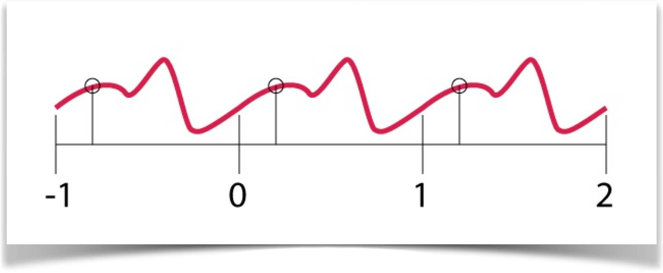
If you give the curve routines a value of t outside of [0,1], you get back the value youd see if the pattern simply repeated forever. For example, as shown below, t=1.2 is the same as t=.2 , and t=-0.8.
Many (though not all) of the saves contain a parameter that allows you to control some aspect of the waves shape. I've arbitrarily named that parameter a in this library. Values of a are clamped to [0,1]. In other words, values of a less than 0 are interpreted as 0, and values greater than 1 are interpreted as 1.
Note that if you want to use the wave to create endlessly repeating results that look smooth, you'll want the wave to be continuous. In this context, that means two things. First, you need to be able to draw a complete cycle without lifting your pencil from the paper (for example, the triangle satisfies this, but the box does not). Second, you need to make sure that the value at t=1 matches the value at t=0, so the wave repeats seamlessly.
Well see that for some of the curves, some values of a will cause the values at t=0 and t=1 to be different. So when the cycle repeats, whatever you're controlling with the curves value will change suddenly, and usually this is attention-grabbing. For example, if you're using the wave to control the location of something on the screen, a sudden change in value will cause the object to suddenly teleport to the new location. Sometimes this kind of discontinuity is desirable, so I make it available, but use it with care.
Another thing that's easily noticed is a corner, or any place where the curve suddenly changes direction (for more on this subject, see Imaginary Institute Tech Note #3, Blending and Easing). For now, just note that using a wave with corners will result in something that looks more artificial than natural, full of sudden changes. Those changes will also grab your audiences attention, so you need to be careful how you use them.
Generally speaking, for natural motion, you'll want to use waves that are both continuous and smooth. But you'll find lots of times when you want non-continuous or non-smooth curves (or both!), so you'll find them easy to create as well.
To get the value for any wave in this library, there's exactly one function call to know:
float getWave(int waveType, float t, float a);
Here are your choices for waveType, all discussed in detail below:
- WAVE_TRIANGLE
- WAVE_BOX
- WAVE_SAWTOOTH
- WAVE_SINE
- WAVE_COSINE
- WAVE_BLOB
- WAVE_VAR_BLOB
- WAVE_BIAS
- WAVE_GAIN
- WAVE_SYM_BLOB
- WAVE_SYM_VAR_BLOB
- WAVE_SYM_BIAS
- WAVE_SYM_GAIN
Along with the wave type, you provide the values for t and a , and back comes the value of the named curve, as shaped by a , at the value of t . When you use these values, precede them with AULib and a period, as in this example:
float myValue = AULib.getWave(AULib.WAVE_BOX, .5, .5);
The Waves
In the following sections, each wave is drawn three times, so you get a feeling for how it looks when it repeats. To draw these plots, I just ran t from 0 to 3. So the first third is the wave as defined, from t=0 to t=1. The middle third is the first repeat, from t=1 to t=2, and the next third is the second repeat, from t=2 to t=3. You can keep the curve repeating forever by using ever-larger values of t .
Triangle
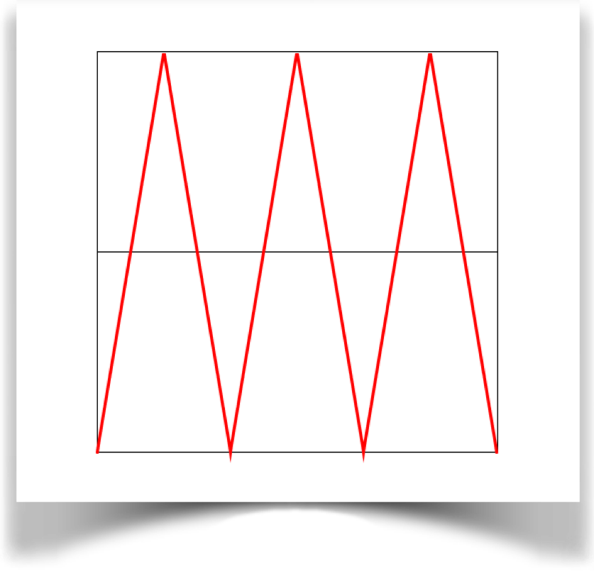
The triangle wave is specified with the type WAVE_TRIANGLE.
This wave starts at 0 at t=0, rises up in a straight line to a value of 1 at t=.5, and comes back to 0 at t=1. . This wave is continuous, but it has an eye-catching corner each time it changes direction.
The a variable has no effect on this wave.
Box
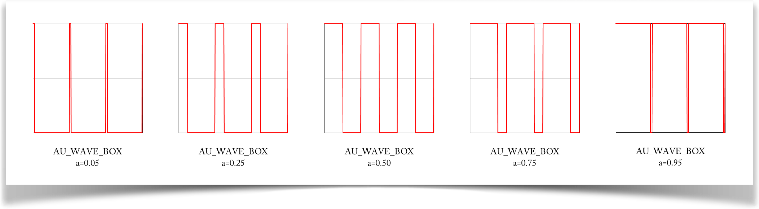
The box wave is specified with the type WAVE_BOX.
At t=0, the curve starts with a value of 1. It stays at 1 until t=a, when it jumps down to a value of 0, and stays there for the rest of the wave. This curve is not continuous, because it jumps twice (up to 1 and down to 1). And it has corners at each jump. Thus, this wave looks very mechanical and inorganic.The value of a identifies the value of t where the curve switches from a value of 1 to a value of 0.
Sawtooth
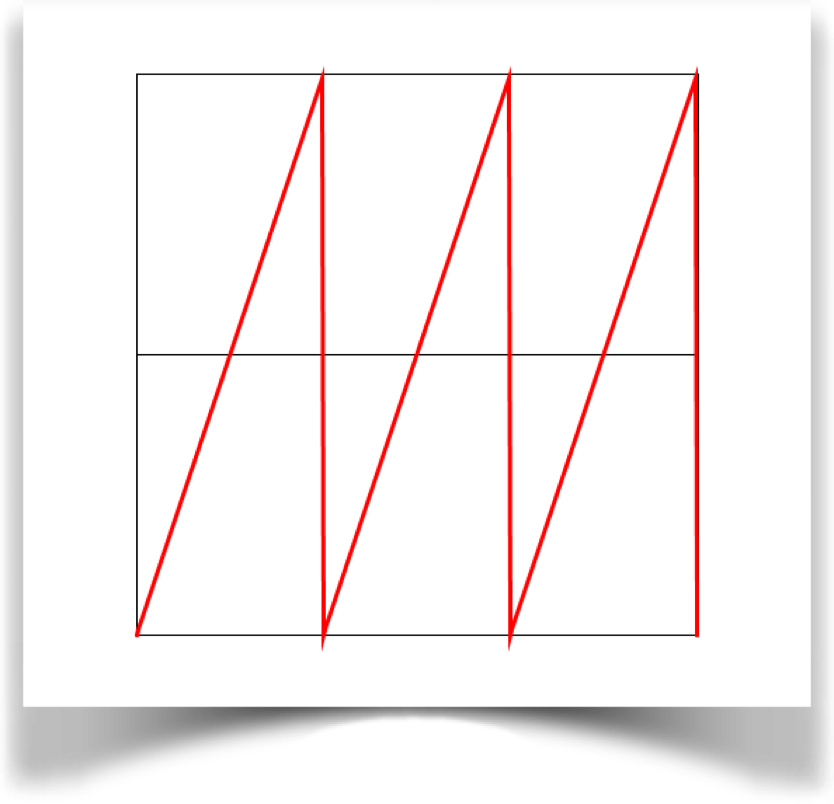
The sawtooth wave is specified with the type WAVE_SAWTOOTH.
Here we start at 0 when t=0, and rise in a straight line to 1 at t=1. In other words, the value of the curve is just the value of t. It is not continuous, because it leaps suddenly from 1 to 0 on each repeat. It also has corners at that transition point.
The a parameter has no effect on this wave.
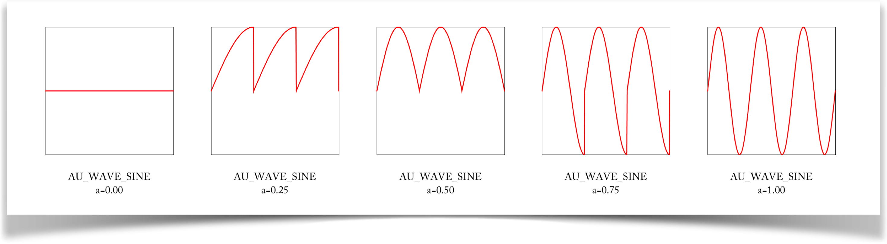
Sine
The sine wave is specified with the type WAVE_SINE.
Suppose a has the value 1. Then this curve starts at .5 and smoothly rises to 1 at t=.25, where it smoothly changes direction, drops back through .5 again at t=.5, and drops to 0 at t=.75, where again it smoothly changes direction and heads back up to .5 at t=1. This curve is continuous, and perfectly smooth: it repeats forever without any jumps or sudden motions. Its based on a function from trigonometry called the sine (see Imaginary Institute Tech Note 02, Trig for CG), though it's adjusted a bit to fit our input and output ranges of [0, 1].
The value of a tells the curve how far to run during the interval from t=0 to t=1 So if a=.5, a single cycle uses only the first half of the sine curve, and that repeats over and over. The a=.5 curve is continuous, but it has a corner each time it changes direction. Other values of a work the same way. For example, a value of a=.25 means a single cycle only occupies the first quarter of the sine curve. A value of a=0 means the curve never even moves from its starting value of 0.5. The odds are pretty good that you'll probably use a=1.0 0 almost all the time, a=0.5 a little bit, and other values very rarely.
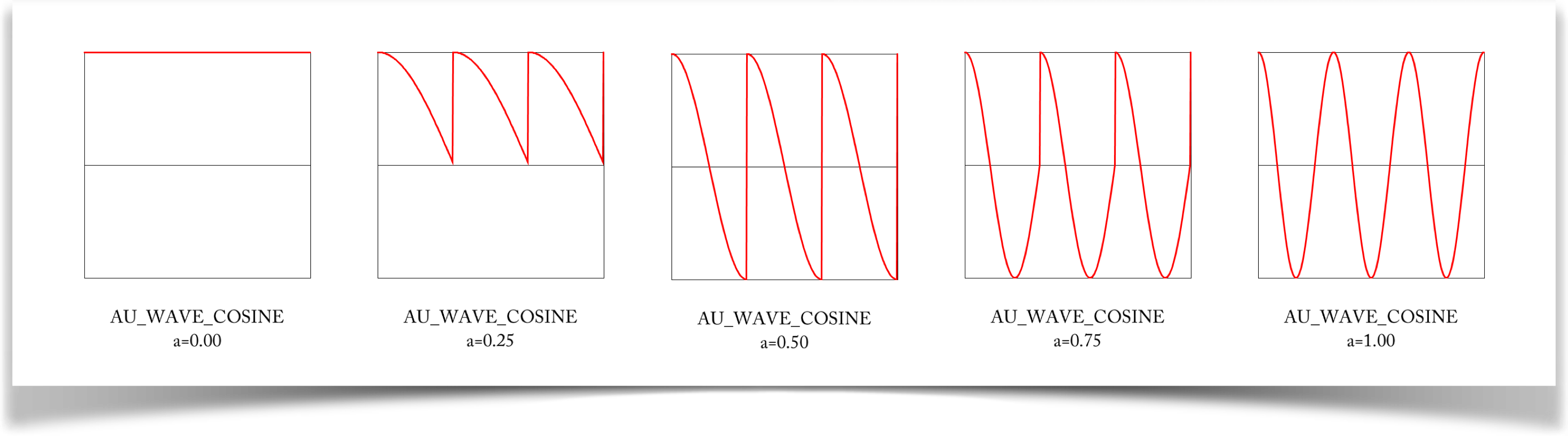
Cosine
The cosine wave is specified with the type WAVE_COSINE.
The cosine is exactly like the sine, only its shifted by 1/4 wave. Thus a single cycle starts at 1, drops to 0, and rises again to 1. It is also continuous and super-smooth, because it really is literally just the sine curve but shifted over a little.
The a parameter works the same way as for the sine: it tells you how much of the cosine curve to use for each cycle of this wave. And as with sine, youull probably use a=1.0 almost all the time, a=0.5 a little bit, and other values very rarely.
Blob
The blob wave is specified with the type WAVE_BLOB.
This curve starts at 1 when t=0, and drops down smoothly to 0 when t=1. It's called a blob curve because it was the mathematical heart of a technique for drawing object that were jokingly called blobby objects. It's better known in most of math and science as the Gaussian curve, or the bell curve.
The a parameter has no value on this wave.
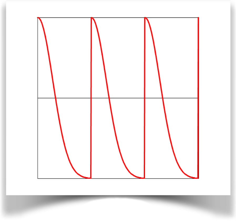
If this doesn't look like any blob functions you're used to, remember that this were drawing only the right side (that is, for t>0). Below well see how to produce a more familiar, symmetric version.
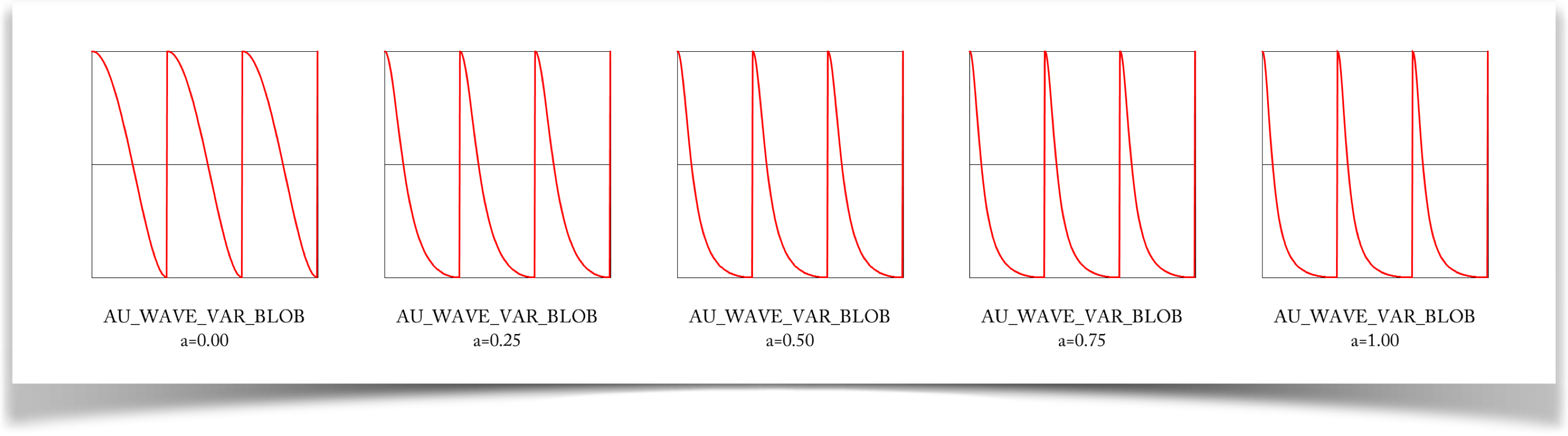
Variable Blob
The variable blob wave is specified with the type WAVE_VAR_BLOB.
This curve is very like the blob, but it allows you some control.
The a parameter controls how quickly the curve drops from 1 to 0. The value of a can go as low as 0, but as high as you like. When its near zero, that means that the curve changes slowly, giving us a shape like the bell curve. As you crank up the value of a, the curve drops off sooner and sooner, spending more of its time slowing down to 0.
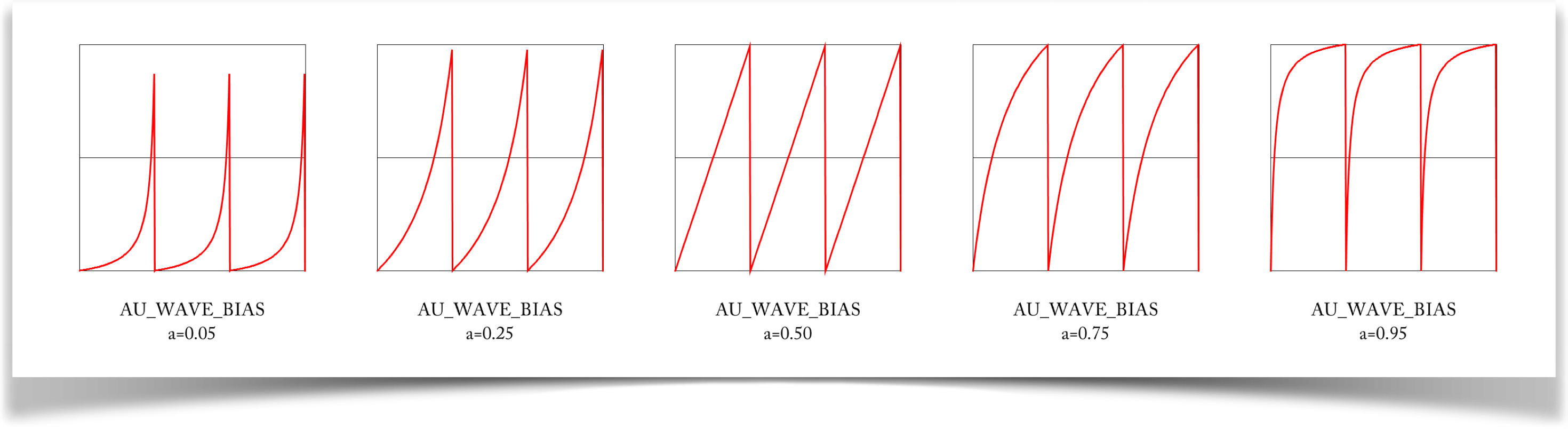
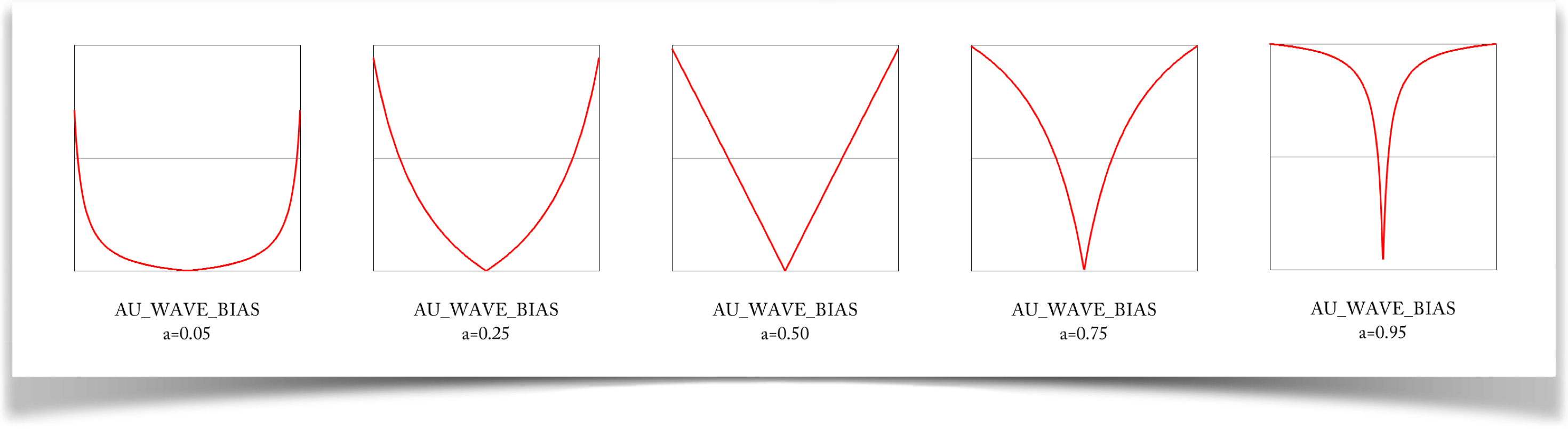
Bias
The bias wave is specified with the type WAVE_BIAS.
The bias curve starts at 0 when t=0 and ends at 1 when t=1, but what happens in between is entirely dependent on the parameter a.
When a is very nearly 0, the curve starts out slowly, and then picks up speed. Note that this slow start is not smooth: there is a corner at the start of each cycle. As you increase the value of a , this slow start picks up speed. When a=.5, the curve is flat, just like the sawtooth. As a continues to rise, the starting speed continues to rise as well, causing the curve to flatten out as it reaches 1. When a is nearly 1, the curve is basically a sharp rise to nearly 1, and then a slow ascent the rest of the way.
The extreme values of a don't do much: a=0 gives us a constant output of 0, while a=1 gives us a constant value of 1. The interesting values are between these extremes.
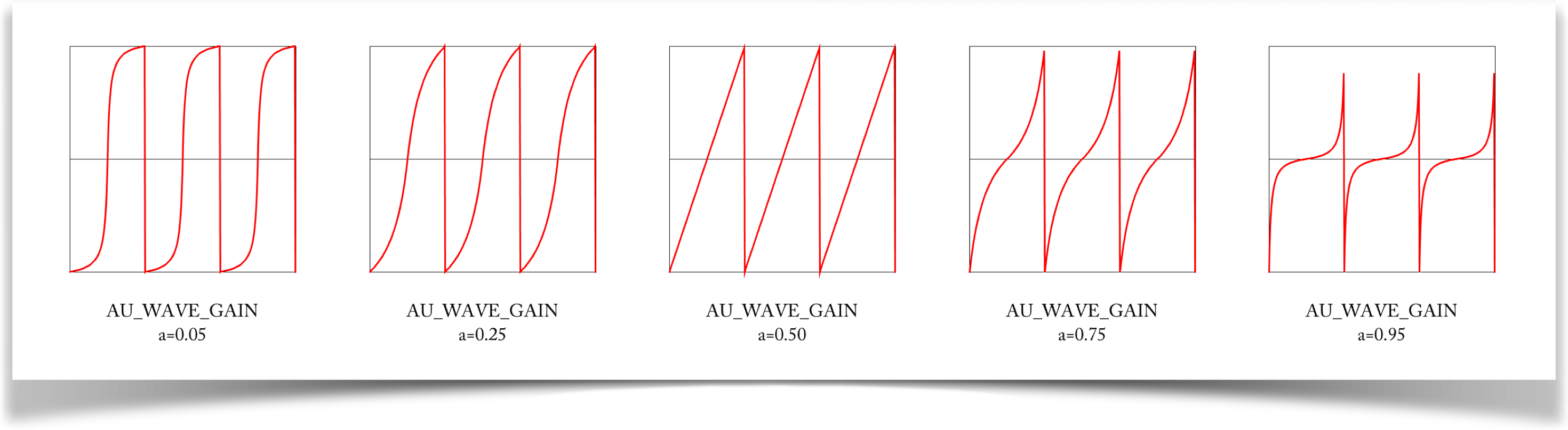
Gain
The gain wave is specified with the type WAVE_GAIN.
The gain curve is like two bias curves stitched together, making a kind of S curve. As with bias, the shape of the curve is dependent on a. The curve is symmetrical about the center, with a value of 0.5 at t=0.5.
When a is very small, the curve rises slowly from 0, jumps (but smoothly) to nearly 1, and then slowly settles into 1. Larger values give more gentle S shapes, until we get a straight line at a=.5. Larger values of a give even steeper starts, slower growth near the middle, and then a steeper end.
As with bias, the extreme values of a don't do much: a=0 gives us a constant value of 0, while a=1 gives us a constant value of 0.5. The interesting values are between these extremes.
Symmetric Waves
Some of these waves have a particularly useful form when we make them symmetric around t=0. The first few waves don't look all that different, but the last four are worth noting. Here is a single cycle of each of them.
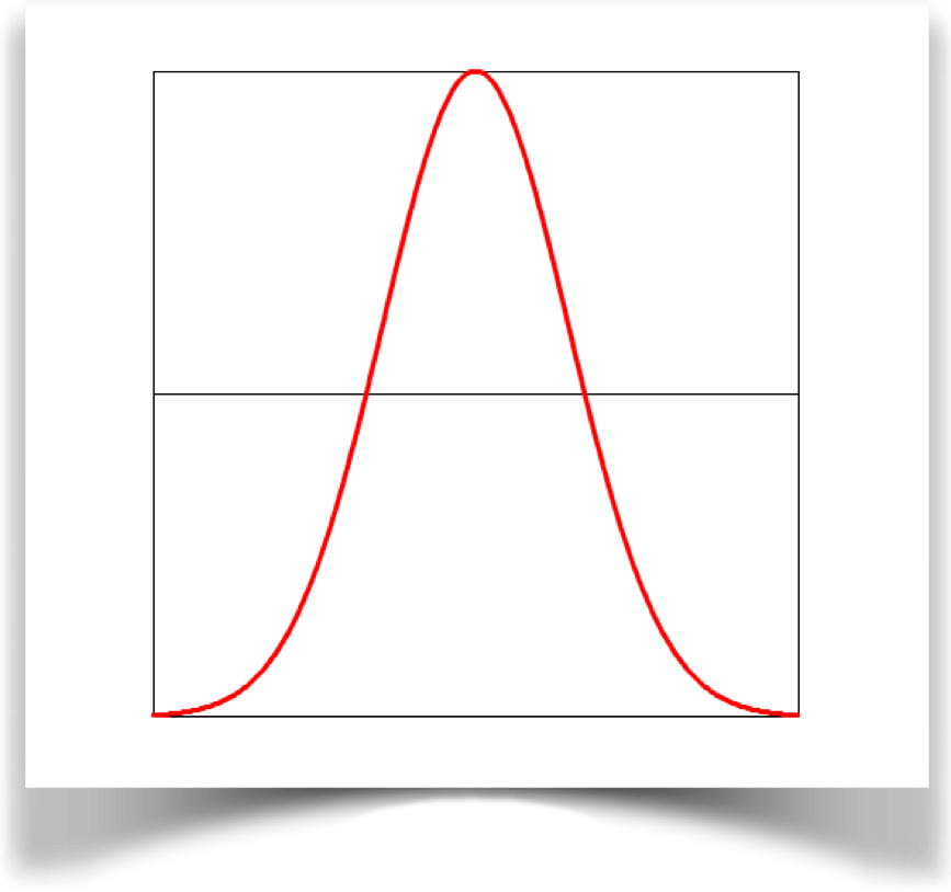
Symmetric Blob
Here's the symmetric blob, which is generated by the type WAVE_SYM_BLOB. Now it looks like the famous Gaussian bump, or bell curve, which lies at the heart of huge swaths of mathematics, science, and engineering:
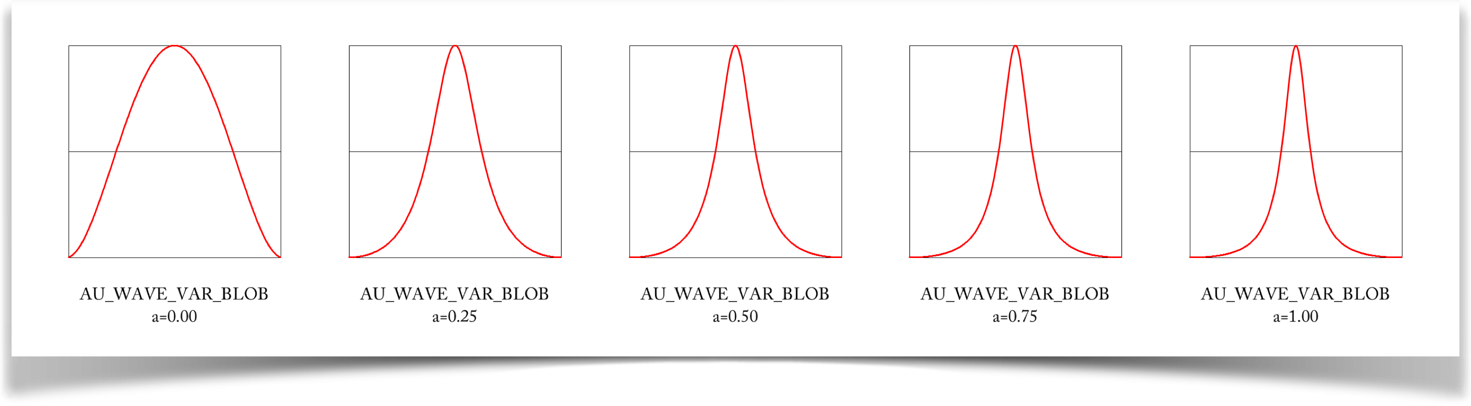
Symmetric Variable Blob
The symmetric variable blob produced by type WAVE_SYM_VAR_BLOB. The symmetric variable blob is just like the regular variable blob, but of course we can control its shape:
Variable Bias
The variable bias curve, produced by type WAVE_SYM_BIAS, gives us an interesting range of shapes:
Symmetric Gain
The symmetric gain curves are produced by the type WAVE_SYM_GAIN. They're pretty attractive, too, and offer lots of interesting shapes for controlling motion: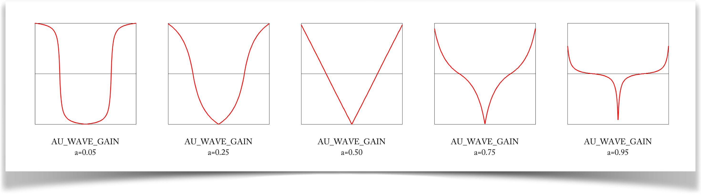
Tech Talk
Here are some details on the waves provided by the library. None of this is necessary for using the library, so you can skip this section if you're not into the math and programming side of things.
The Waves
Here's the math behind the waves. For pictures of these functions, look back at the previous sections.
The first 5 waves are all straightforward mathematically.
WAVE_TRIANGLE
$$ v = 1 - (2 | t-.5| ) $$WAVE_BOX
$$ v = \begin{cases} \rm{if\;} t \in [0,a] & 1 \\ \rm{else} & 0 \end{cases} $$WAVE_SAWTOOTH
$$ v = t $$WAVE_SINE
$$ v = (1 + \sin(2 a \pi t))/2 $$WAVE_COSINE
$$ v = (1 + \cos(2 a \pi t))/2 $$WAVE_BLOB
The interesting thing about the blob is that there are lots of blobs to choose from! Here is a short list of candidate functions that have all appeared in the computer graphics literature as candidates for something like the Gaussian curve (note that when you code these, you can rearrange some of them to save a few multiplies. I'm presenting them here in their expanded form, since I think it's easier to see what's going on that way):
Blinn
$$ v = \frac{e^{-4t^2}-e^{-4}}{1-e^{-4}} $$Nishimura et al
$$ v = \begin{cases} \rm{if \;} t < 1/3 & 1-3 t^2 \\ \rm{else\;} & .5(1-t)^2 \end{cases} $$Wyvill et al.
$$ v = \frac{-4 t^6 + 17 t^4 - 22 t^2 + 1}{9} $$RenderMan
$$ v = -t^6 + 3 t^4 - 3t^2 + 1 $$Baranoski/Rokne:/h5>
This function has an additional parameter, $t$, which allows you to adjust its shape: $$ v = \frac{(t-1)^2 (t+1)^2}{1+dt^2} $$
Cosine
$$ v = .5(1+\cos(2\pi t)) $$Discussion
The Blinn function is a Gaussian that's been modified so that it really goes to 0 at t=1 (rather than very close to zero). The others are all very similar. One option, Barnoski/Rokne, includes an additional parameter (which they called d that allows you to adjust the shape of the curve.
Here are all half-dozen curves all plotted on top of one another. For the Baranoski/Rokne curve I set d to 1.4:
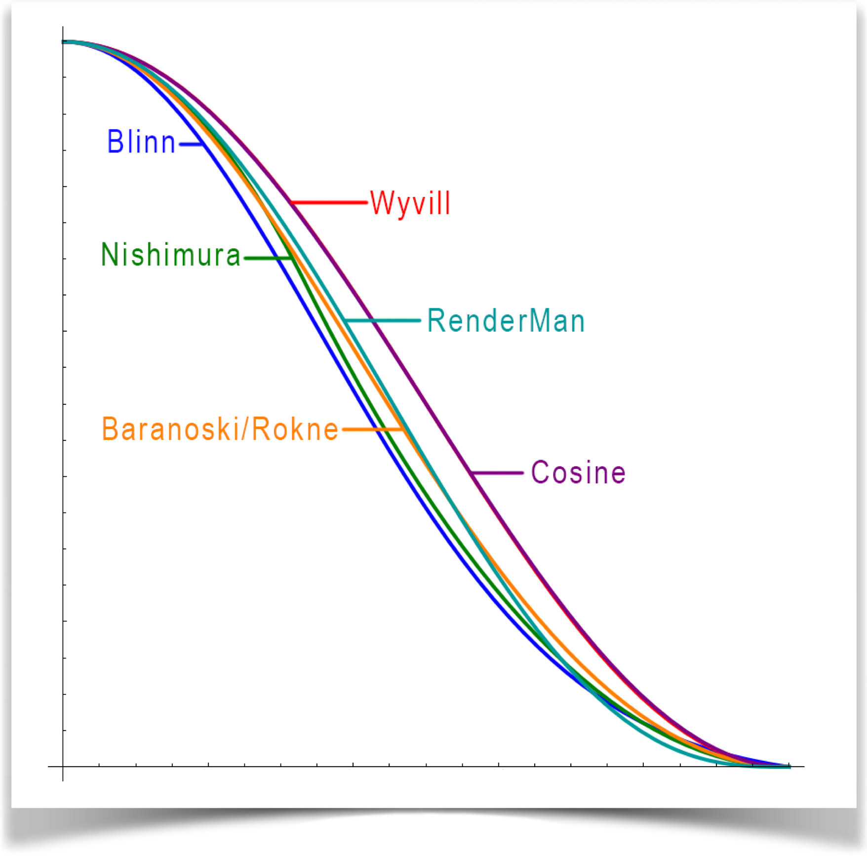
They're all very similar, so the visual differences between the results will all be pretty small. And since you'll usually tune and tweak your results to look just right to you, it really doesn't matter a lot which one you use. So for this library I went with the classical choice and selected a Gaussian curve, adjusted in the same style as Blinns function.
Blinn's curve tails off at 2 units from the origin (each 4 in that equation is actually 22). So at t=1, his curve has a derivative of about .018, which is larger than 1/255 (about .004). So there's a tiny chance of seeing a little Mach band if you use this function for color gradients. So I extended the curve to 2.5, where the derivative drops to about .002, eliminating that potential problem.
In conclusion, Here's the equation defining the WAVE_BLOB in the library:
$$ v = \frac{e^{-{(2.5t)^2}}-k} {1-k} {\rm\;\;\;where\;\;\;} k = e^{{-2.5}^2} $$WAVE_VAR_BLOB
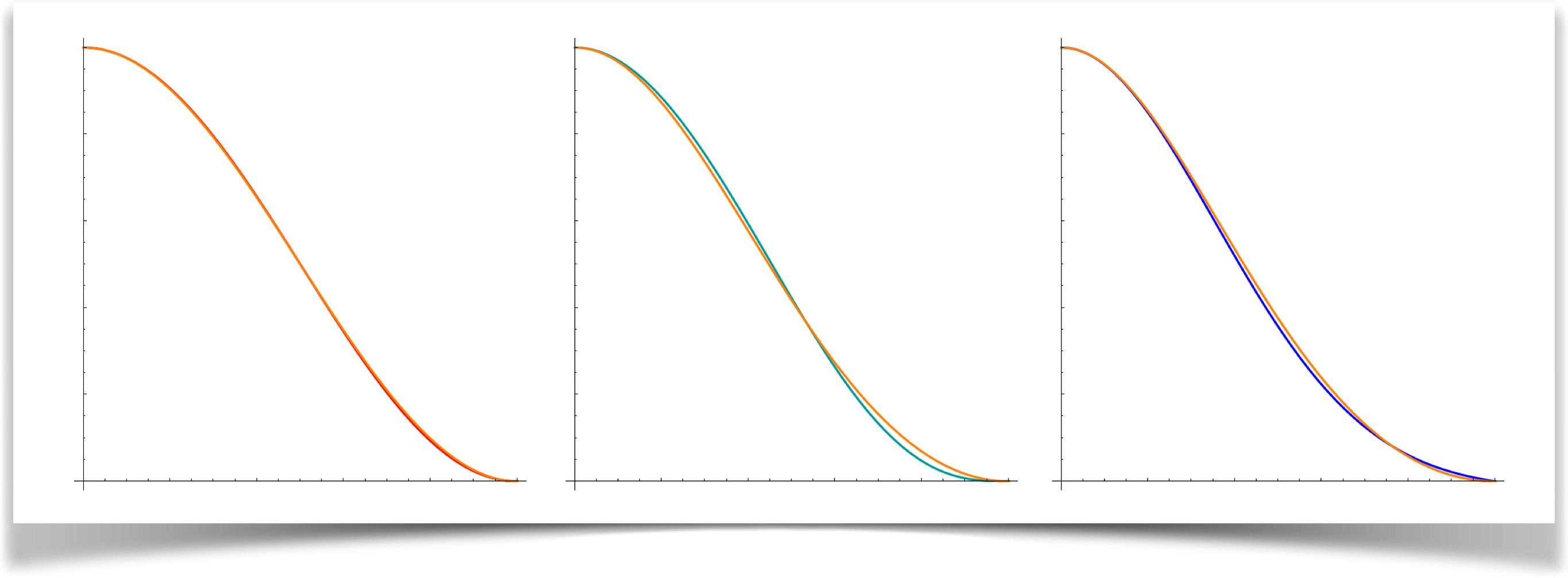
Although I went with the classical Gaussian for the blob, I really liked the idea of being able to tune the shape of the blob. So I also provide the Baranoski/Rokne formula. The value a that is passed into the function is used for the tuning parameter, written d in the equations above. It must be greater than -1. As a increases, the central core becomes thinner and thinner.
$$ v = \frac{(t-1)^2 (t+1)^2}{1+at^2} $$Visually, when a=0.5 this is just about identical to Wyvill/cosine. At about a=1.4, it's close to the RenderMan curve. When a=1, it's very similar to the Blinn curve.
WAVE_BIAS
There's a long history of various functions that bend downward or upward. Perlin suggested a pair of functions that he called bias and gain that became popular, and the names stuck. Schlick developed simpler and more efficient versions, and those are what I used here. For both the bias and gain, we make the notation easier with three helper variables: $$ j = \frac{1}{a}-2, \;\;\; k = 1-2 t, \;\;\; s = jk $$ Note that $j$ depends on $a$, our control variable. With these variables, the bias is $$ v = \frac{t}{j(1-t)+1} $$WAVE_GAIN
Using the same variables $j$ and $k$ above, the gain is given by:
$$ v = \begin{cases} \rm{if\;\;} t<.5 & t/(s+1) \\ \rm{else\;\;} & (s-t)/(s-1) \end{cases} $$Resources and References
The library, examples, documentation, and download links are all at the Imaginary Institutes resources page:
https://www.imaginary-institute.com/resources.php
To use it in a sketch, remember to include the library in your program by putting
import AULib.*;
at the top of your code. You can put it there by choosing Sketch>Import Library... and then choosing Andrew's Utilities, or you can type it yourself.
This document describes only section of the AU library, which offers many other features. For an overview of the entire library, see Imaginary Institute Technical Note 3, The AU Library.
Here are the sources for the various blob functions described above.
James F. Blinn, "A Generalization of Algebraic Surface Drawing", ACM Transactions on Graphics, July 1982
Fujita, T., Hirota, K. and Murakami, K., "Representation of Splashing Water using Metaball Model", Fujitsu, 1990, Vol 41, part 2, pp 159-165
G. Wyvill, C. McPheeters,C. Wyvill, "Data Structure for Soft Objects", The Visual Computer, 2(4), pp. 227-234, 1986.
Gladimir V. G. Baranoski and Jon Rokne, "An Efficient and Controllable Blob Function", Journal of Graphics Tools, Volume 6 Issue 4, 2002, Pages 41-54
Blobby Implicit Surfaces, "PhotoRealistic RenderMan Application Note #31", http://renderman.pixar.com/resources/current/rps/appnote.31.html
Ken Perlin, "An Image Synthesizer", Computer Graphics (Proc. SIGGRAPH 1985), v19 n3, p 183-190, 1985
Christophe Schlick, "Fast Alternatives to Perlins Bias and Gain Functions", Graphics Gems IV, ed. Paul Heckbert, Academic Press