The AU Library:
Equal Spacing Along Curves

Andrew Glassner
https://The Imaginary Institute
15 October 2014

andrew@imaginary-institute.com
https://www.imaginary-institute.com
http://www.glassner.com
@AndrewGlassner

Imaginary Institute Tech Note #8

Table of Contents

• Introduction
• AUCurve
• AUBezier
• Getting Curve Values
• Setting Curve Values
• Tangents
• Examples
• Mixing your curves with AUBaseCurve
• Tech Talk
• Resources

Introduction

Curves are important in graphics. We use them not only for drawing smoothly flowing shapes on the screen, but for controlling how objects move and how they change over time.

Processing offers two different types of curves, each named for the people who developed their mathematics and popularized their use: Catmull-Rom curves, and Bezier curves. The Catmull-Rom functions have the word curve in them, while the Bezier-related functions have the word bezier in them.

There's a lot to know about how to create, manipulate, and use curves. In this note I'll assume you're already familiar with both of these kinds of curves, how they're used, and how to create complex curves by smoothly stitching together many simpler curves.

The purpose of this note is to present a couple of objects designed to help you with just one job: creating equally-spaced points along either of these curves.

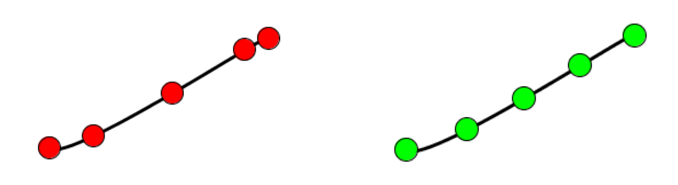
You might think that this is easy. For example, to draw five equally-spaced circles along a Catmull-Rom curve, you might try evaluating the curve at five equally-spaced values of the interpolation parameter t, writing a loop like this:

for (int i=0; i<5; i++) {
  float t = i * 0.25;
  float x = curvePoint(100, 400, 200, 300, t);
  float y = curvePoint(400, 200, 300, 100, t);
}

The result is shown below on the left. Note that the points are not equally spaced, even though the parameter values were. In fact, you'll almost never get equally-spaced points from this technique. What we want is on the right.

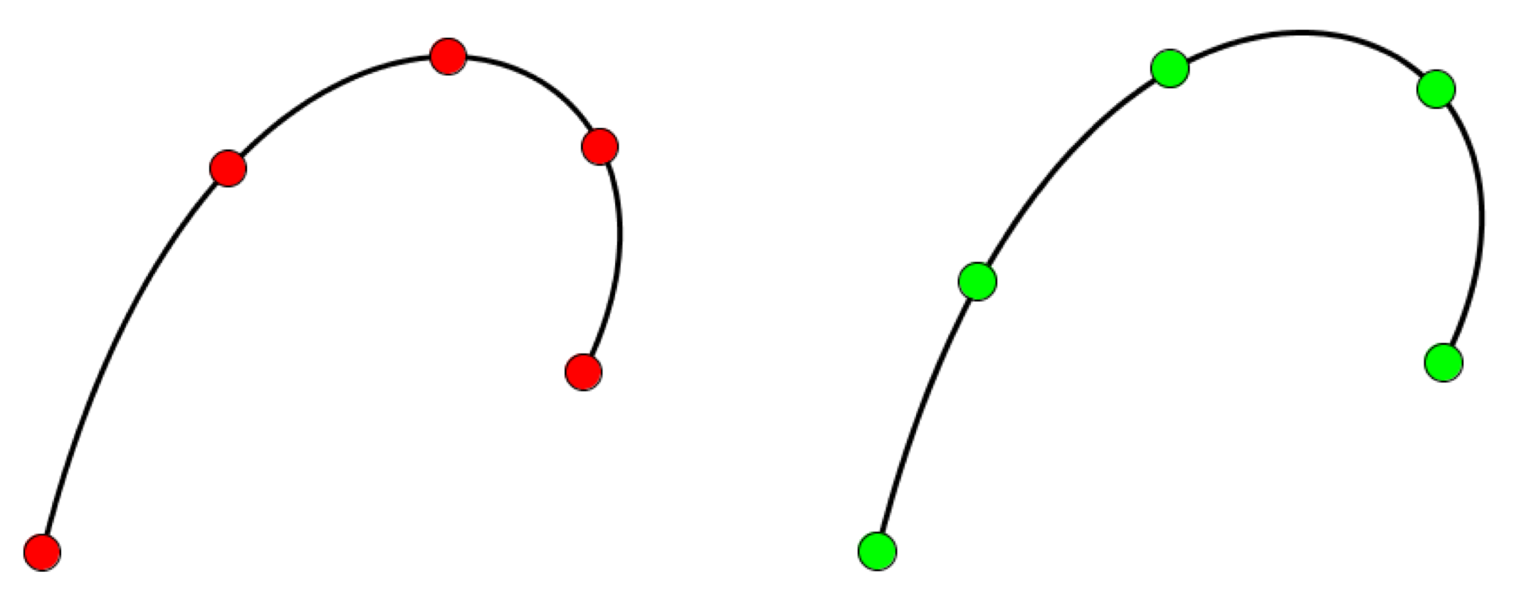
This isn't just a problem with Catmull-Rom curves. Bezier curves have the same problem, as in the next figure.

This isn't evidence of something wrong in Processing, Java, or the graphics libraries they use, or anything else. It's a natural result of the mathematics of the curves. The equations that generate these smoothly-flowing curves were not designed to ensure that equally-spaced parameter values would produce equally-spaced points, and, most of the time, they don't. Technically, we say that the points are produced parametrically, rather than as functions of arc length, or distance measured along the curve.

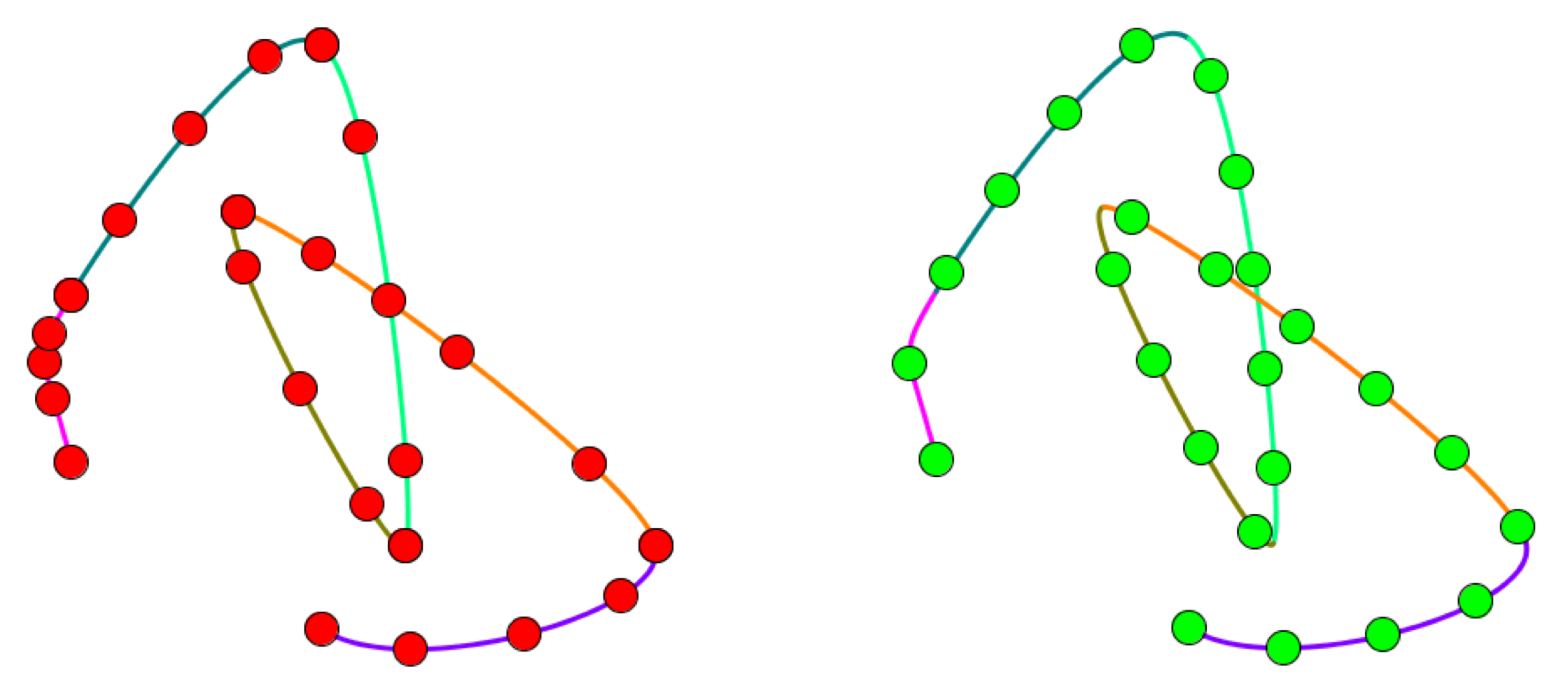
To make the problem worse, suppose you stitch together several curves to make one large curve, and you want to generate equally-spaced points along the larger curve. Without doing a lot of work, this seems nearly impossible. One approach might be to put a constant number of points on each subcurve, but that doesn't turn out well. The results are shown here for Catmull-Rom curves, along with the solution we'd prefer.

Note that if were just drawing our curves, we don't care about this spacing stuff. Processing takes care of this variation in spacing for us, and makes sure that the drawn curve looks nice and smooth.

But if were using the curve to control motion, this can be a real problem. We might want an object to move from one place on the screen to another, so we create a curve and we get points along the path to position the object over time. But rather than moving at a constant speed, it would speed up and slow down in ways that we can't control.

Similarly, if were placing objects along the curve, like little lights along a wire, they will usually seem to bunch up and spread out.

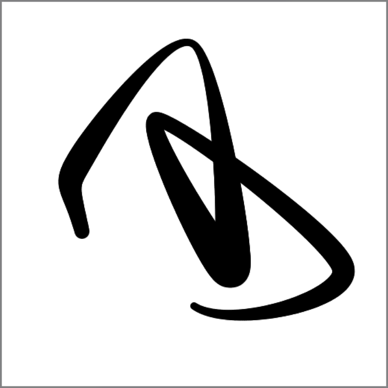
For example, suppose we want to draw a little circle flying around on a big complicated curve made out of lots of segments. We'd like to draw a trail behind the circle on every frame, as shown here.

Using only Processing's built-in tools, the tail would seem to grow and shrink as the circle moved around, and the tail would even seem to have weird changes in its shape when it crossed over a shorter segment to a long one, or vice-versa. Keeping it to a fixed length would take a lot of work.

To resolve these problems, you can use two objects provided in the AU library. There's one object for Catmull-Rom curves and one for Bezier curves. You create these objects by handing them the points that make up your curve, whether its just one segment or a whole bunch of them. Then you ask for points at values of the parameter t , just like with Processing's built-in routines.

But when you use these objects, think of your parameter t as a percentage along the curve. So t=0 represents the point at the start of the curve, t=0.25 is a quarter of the distance along the curve, t=.5 is halfway, and so on, with t=1 the point at the end of the curve.

The library lets you manage curves that are one-dimensional (that is, a single value for each value of t), 2D (like in the figures above), 3D, or in fact as many dimensions as you like.

As an extra bonus, you can include other floats at every knot, and they get interpolated as well. For example, you can include a float with a 2D curve and use that to control the thickness of the stroke. I drew the curve below by attaching a thickness parameter to each knot, and then I drew lots and lots of small circles along the length of the curve, like our demonstrations above. They're so closely spaced that they overlap a lot and the curve looks like a single solid stroke. It wasn't so important in this case that the centers of the circles were equally-spaced, because I was drawing so many of them, but it didn't hurt.

This technique of attaching extra data to each knot lets you easily create gradients and other effects that vary with time, distance, or location.

The library provides you with two objects, one for Catmull-Rom curves, and the other for Bezier curves. Once they're made, you use both kinds of curves in exactly the same way.

Well discuss Catmull-Rom constructors first, then Bezier, and then well look at the things you can do with both of these objects. Of course, getting back points at any desired location along their length will be our primary focus.

AUCurve

The AUCurve object helps us make equally-spaced points along Catmull-Rom curves (what Processing generically refers to as a curve). We create the curve by giving it the points that make up the curve, and then we use that object to convert native parameter values into uniform parameter values.

Creating

There are three constructors: one each for basic, one-segment 2D and 3D curves, and one much more general constructor that lets you get at the full power of the library.

Here's the 2D constructor:

public AUCurve(float x0, float y0, float x1, float y1, float x2, float y2, float x3, float y3);

The 3D version is the same, except you include a z value in your data:

public AUCurve(float x0, float y0, float z0, float x1, float y1, float z1,
               float x2, float y2, float z2, float x3, float y3, float z3);

For example, to build our curve from the first figure above, youd write

AUCurve myCurve = new AUCurve(100, 400, 400, 200, 200, 300, 300, 100); 

The more general constructor requires a little more attention from you, but it lets you work with big multi-segment curves, and it lets you interpolate other data along with the points:

public AUCurve(float[][] knots, int numGeomVals, boolean makeClosed);

Let's look at these arguments one by one.

First comes knots, a 2D array of floats. Think of this as a vertical list of rows. Each row must begin with your knots position information, typically a float for x and another for y. But you can make these rows as long as you like. Whatever other numbers you include will get interpolated along with the knot values. What you do with these numbers is up to you.

For example, you might include two more floats in each row, one representing the thickness of the curve at that point, and another representing the temperature of the day when that data point was measured. When you ask the curve to evaluate itself at a given value of t, you can get back not just the curves position, but the value of these other floats as well.

Augmenting our data from above with this information, we could create the array like this:

// values are x, y, stroke thickness, temperature
float[][] myKnots = {
  { 100, 400, 6, 60 }, 
  { 400, 200, 7, 70 }, 
  { 200, 300, 5, 80 },
  { 300, 100, 3, 70 }
}; 

This raises a question: how does the library know how many of your entries are geometric, and how many are other things? The questions important because were using the input value of t to determine how far along the curve weve traveled. To get that distance right, our calculations should ignore that non-geometric data (like stroke weight, or temperature, or whatever you're using the other floats to represent).

The argument numGeomVals provides this information. If you have a 2D curve (where the first two values at each knot are x and y), then this argument should be 2. If you have a 3D curve, it should be 3. You always need to provide this value.

Finally, makeClosed does what you think it does: it takes your curve and closes it smoothly. It does this by drawing three extra curve segments, all derived from your data. In the left of the figure I show an open Catmull-Rom curve made up of three segments, along with the knots that define it, numbered 0 through 5. To close the curve, we include the segments formed by knots (3,4,5,0), (4,5,0,1), and (5,0,1,2), as in the right of the figure below.

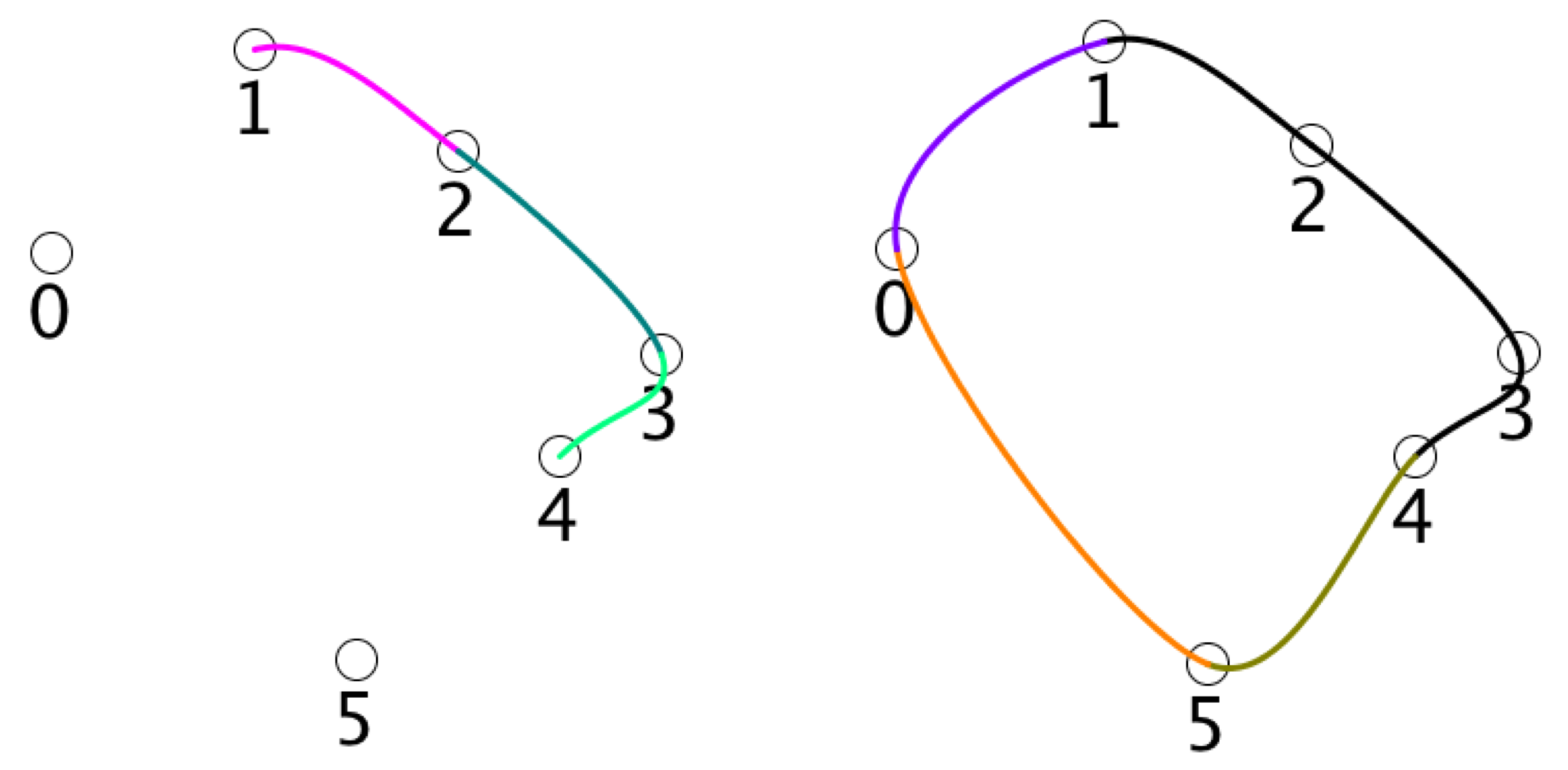
When you tell the system that a curve is closed, the points at t=0 and t=1 are the same. This can cause a little confusion if you're counting the points along your curve.

For example, suppose you have an open curve and you draw 11 equally-spaced circles (using t=0,.1,.2,... 1.0 ). Then you'll see 11 circles on your curve. If you use the same 11 values of t for a closed curve, you'll see only 10 circles, because the circles for t=0 and t=1 are at the same point.

If you've attached other floats to your curve, they get smoothly closed in the same fashion, so they will also join up in a smooth and seamless way.

Curves of Other Than Two Dimensions

If you have only one value to interpolate, each row of your knots array will be only one element. For example, suppose you want to interpolate the amount of red in some object's color over time. You have the values (10, 50, 200, 150, 100) at five evenly-spaced frames. Then you would create this array:

float[][] myKnots = {{10}, {50}, {200}, {150}, {100}};

And use a value of 1 for numGeomVals when you make the curve. Then you can simply use getX() to get the value for any frame.

A Note About curveTightness() and curveDetail()

Processing offers the function curveTightness() to give you control the shape of all your Catmull-Rom curves. Because my library doesn't use Processing's built-in routines to compute points on curves, this function call has no effect on AUCurve objects, or the points they produce.

Similarly, Processing's curveDetail() controls the accuracy of how one of the renderers draws curves. It also has no effect on the curves represented by AUCurve objects. This also applies to bezierDetail() for Bezier curves, discussed next.

AUBezier

The AUBezier object helps us make equally-spaced points along Bezier curves. Everything about it is the same as for the AUCurve above, except the mechanics of how closed curves are handled. I'll assume you've read the AUCurve entry above, so here I'll just present the constructors, and then discuss the closing stuff.

Creating

As before, there are three constructors: one each for basic, one-segment 2D and 3D curves, and one much more general constructor that lets you get at the full power of the library.

Here's the 2D constructor:

public AUBezier(float x0, float y0, float x1, float y1, float x2, float y2, float x3, float y3);

The 3D version is the same, except you include a z value in your data:

public AUBezier(float x0, float y0, float z0, float x1, float y1, float z1,
                float x2, float y2, float z2, float x3, float y3, float z3);

Here's the more general constructor:

public AUCurve(float[][] knots, int numGeomVals, boolean makeClosed);

The knots and numGeomVals arguments are the same as for AUCurve , and work the same way.

To close a Bezier curve, the system does a little more work. The figure below shows an open Bezier curve. To close the curve, the system adds two knots and one more segment to your curve. These elements are constructed to smoothly join the last segment and the first, as on the right hand side of the figure.

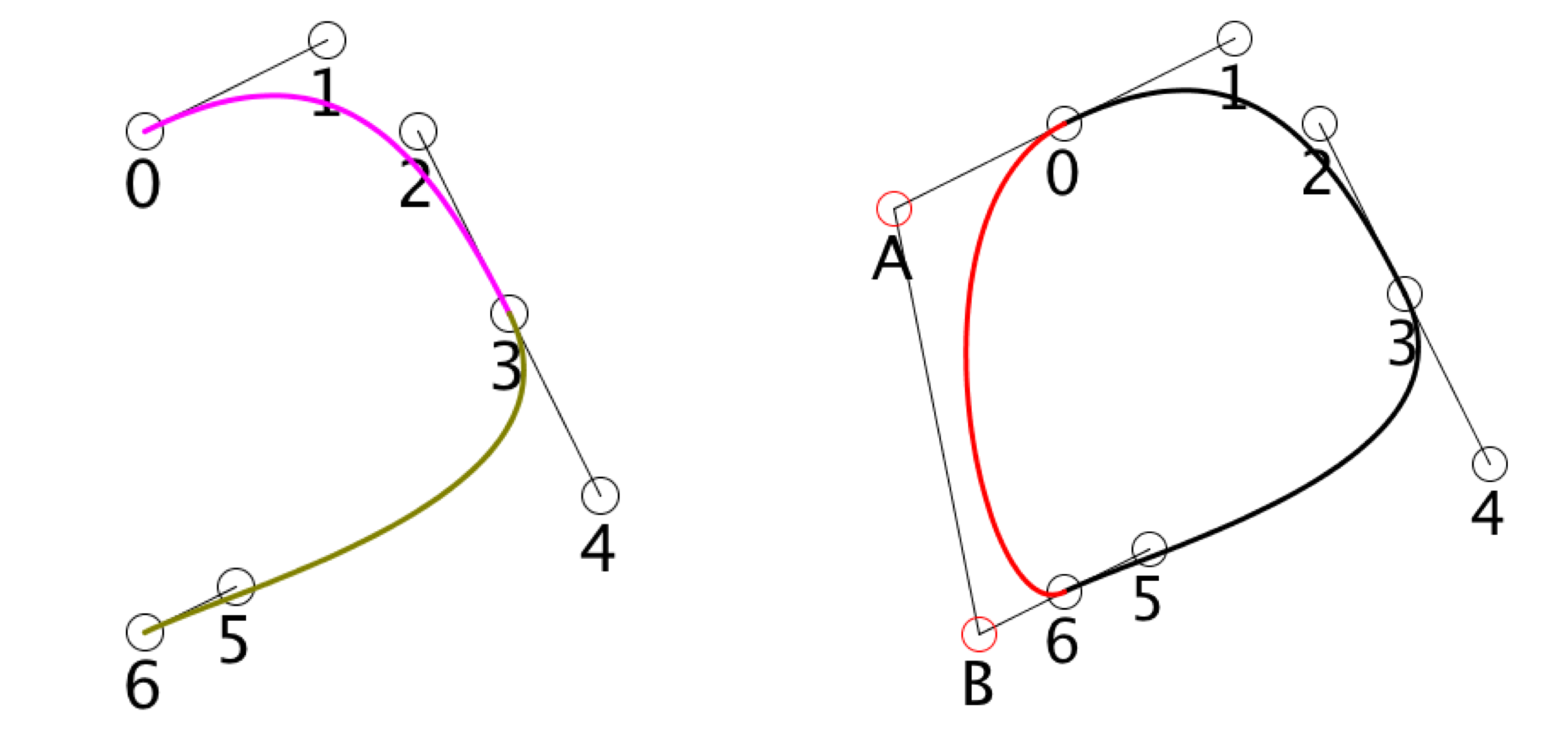
As with the AUCurve , when a curve is closed, the values for t=0 and t=1 identify the same point.

And also, just as with Catmull-Rom curves, if you have other floats attached to your knots (representing, say, thickness, or color, or temperature, or anything else), those will also be blended in this fashion, so they too will join up seamlessly and smoothly.

Getting Curve Values

Once you have either an AUCurve or AUBezier object, you'll want to hand it values of t and get back interpolated values. Remember that in this library, t is a value from 0 to 1 that runs along the entire length of your curve (open or closed), and represents how far along you are as measured along the curve itself . So asking for values at equally-spaced values of t will result in points that are geometrically equally-spaced along the curve.

Because we frequently use 2D and 3D curves, there are shortcuts to get x, y, and z values:

float getX(float t);
float getY(float t);
float getZ(float t);

When you have other data elements in your knots, get at them by providing their index in the array:

float getIndexValue(float t, int index);

In our example above, where temperature was the fourth float on each row, we'd get the interpolated temperature value at time t with getIndexValue(t, 3).

What happens if you ask for data you don't have? For example, you have only two values in each row of your knots array, but you call getZ(), or you have five values in each row, but you ask for index 13? The system could print out an error, but that felt to me like overkill, and in fact could prevent some potentially creative uses of the library.

So if you ask for missing data, the system returns the number 0.

Wrapping t

The curve starts at t=0 and ends at t=1 . What happens if you call one of these routines with a value of t outside that range?

By default, the value of t will wrap around. So t=1.23 will be interpreted as t=0.23 , t=834.7 will be interpreted as t=0.7 , and so on. Negative values work a little differently, but they do what youd expect when you use them. So t= -1.2 is interpreted as t=0.8 , and t= -37.51 is interpreted as t=0.49 .

This makes it very convenient to produce cyclic animations. For example, suppose you want to have your object move around the curve every 120 frames. You could write this

float t = frameCount/120.0;

and everything will work fine. t will start at 0 and go up and up, but only the fractional part will matter when you ask for a value.

Note that I wrote 120.0 rather than 120, to make it a floating-point value. Otherwise Processing will do integer division, and you'll get t=0 for the first 120 frames, then t=1 for the next 120 frames, and so on.

If you prefer to tie your program to its running time using millis() , you could have the object make one circuit every 2 seconds (or 2000 milliseconds) with

float t = millis()/2000.0;

If you don't want this wrapping behavior, you can instead tell the curve to clamp your values of t . Then any value of t that is less than 0 will be treated as 0, and anything larger than 1 will be treated as 1. To enable clamping, call

void setClamping(boolean clamp);
(default = false)

with a value of true. As with all the other routines, this is a property of the curve, so you can make some curves in your program do clamping, and others do the default of wrapping.

If you want to turn clamping off, call setClamping() again with a value of false.

Setting Curve Values

You may want to change your curves knot values on the fly. Of course, you can always create a new AUCurve or AUBezier object if you want. In fact, if you're modifying all the knots in an existing curve, its easiest to simply build a new curve to take the place of the old one.

But if you're making just a few changes, you can instead modify the values in an existing curve.

If you just want to change the x, y, or z value for a single knot, there are shortcuts for that:

void setX(int knotNum, float x );
void setY(int knotNum, float y );
void setZ(int knotNum, float z );

There are also shortcuts for setting both x and y, or all 3 values, at once:

void setXY(int knotNum, float x, float y);
void setXYZ(int knotNum, float x, float y, float z);

You can also set the value of any float in any row, by specifying the knot number, the index you want to change, and the new value:

void setKnotIndexValue(int knotNum, int index, float value);

You could use this instead of the shortcuts above, for example by specifying an index of 0 for your x entry.

You can also set all the values for a whole row at once:

void setKnotValues(int knotNum, float[] vals);

Note that when you change a value, some internal data in the library has to be recomputed as a result. This will usually be so fast you won't notice, but if it becomes an issue, see Section 7 for a discussion of how to speed things up. Happily, you can change lots of values (that is, you can call the above routines) as much as you want without penalty. The system will only actually recompute the data it needs the next time you ask for a value using one of the query routines.

The above procedures let you change a few values here and there. What if you want to change all the values in the entire curve? There's no specific call for that, because a better approach is to simply create a whole new curve by calling a constructor with your new data.

Tangents

You can get tangent information at any point along an AUCurve or AUBezier object. If you're looking for tangents to your geometry data, you can use

float getTanX(float t);
float getTanY(float t);
float getTanZ(float t);

When you have other data elements in your knots, you can find their tangents as well, by identifying which index element you want:

float getIndexTan(float t, int index);

This way you can get tangents to the temperature, or stroke thickness, or rainfall, or whatever other data you miht have stored with your curve.

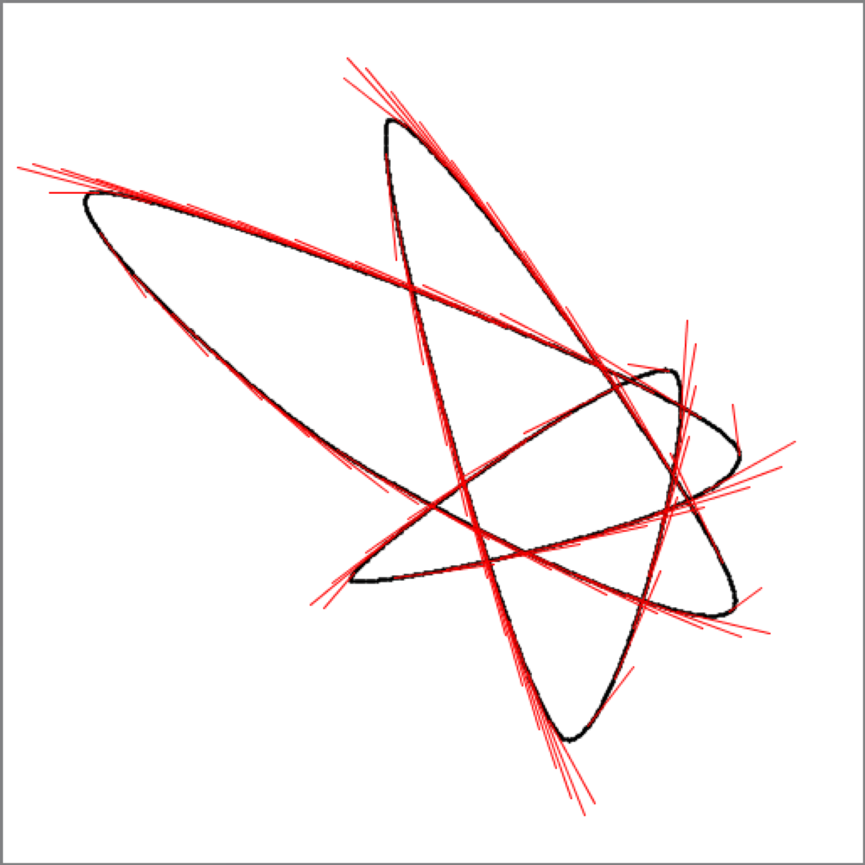
As usual, if the curve is closed, the tangents will follow along. Here's an example of a multi-segment AUCurve with tangents drawn in red (I just drew a red line from each ( (x, y) ) to ( (x+tanx, y+tany) ):

Examples

Here are some examples of using the curve objects in the AU library.

Colorful Thickness-Changing Ropes

The idea here is that we create a random Catmull-Rom curve with a whole bunch of segments. When we create the curve, each knot has not only an x and y value, but it also has four more values: a diameter, and three values for the hue, saturation, and brightness of the curve at that point. Note that the color blends will look smooth across the knots, which you wouldn't get if you used, say, lerpColor() across each segment (your eye would usually pick out the fact that the colors change at different rates when they cross from one curve segment to another; to see why, read up on Mach bands).

To draw the blobby, colorful curve, I just draw a whole lot of equally-spaced dots long the curve. The dot technique is not the fastest way to draw this, but it makes for a good demonstration of using the library.

import AULib.*;

int NumKnots = 8;       // how many knots are in the curve
AUCurve MyCurve;        // the AUCurve itself
boolean Redraw = true;  // only redraw when something's changed

void setup() {
  size(500, 500);
  colorMode(HSB);       // all color operations should be in HSB
  newCurve();           // make a new random curve
}

// draw the curve as a large number of equally-spaced dots
void draw() {
  if (!Redraw) return;  // don't bother redrawing the same thing
  background(255);      // white background
  noStroke();           // dots don't have an outline
  int numSteps = 500;   // how many dots to draw
  for (int i=0; i<numSteps; i++) {
    float t = norm(i, 0, numSteps-1);         // t runs from [0,1]
    float x = MyCurve.getX(t);                // get X at this t
    float y = MyCurve.getY(t);                // get Y at this t
    float diam = MyCurve.getIndexValue(t, 2); // get the diameter
    float hue = MyCurve.getIndexValue(t, 3);  // get the hue
    float sat = MyCurve.getIndexValue(t, 4);  // get the saturation
    float brt = MyCurve.getIndexValue(t, 5);  // get the brightness
    fill(hue, sat, brt);        // fill with this color
    ellipse(x, y, diam, diam);  // draw this dot
  }
  Redraw = false;    // don't draw again until something changes
}

// build a new, random curve
void newCurve() {
  // each knot row: 0:x 1:y 2:weight 3:hue 4:saturation 5:brightness
  float[][] knots = new float[NumKnots][6];   
  for (int i=0; i<knots.length; i++) {
    knots[i][0] = width * random(.2, .8);  // a value for X   
    knots[i][1] = height * random(.2, .8); // a value for Y not
    knots[i][2] = random(5, 50);           // line weight
    knots[i][3] = random(0, 255);          // hue 
    knots[i][4] = random(150, 255);        // saturation
    knots[i][5] = random(150, 255);        // brightness
  }
  /* Make the new curve. Give it the knots, tell it we have 2 
   * geometry values at the start of each row (the X and Y values),
   * and close it. Remember the geometry values must always come 
   * at the start of each row in the knots.
   */
  MyCurve = new AUCurve(knots, 2, true);   
  Redraw = true;    // we have a new curve, so draw it
}

// Give the user some controls. Rebuild and redraw after any changes.
void keyPressed() {
  switch (key) {
    case ' ':
      newCurve();  // make a new curve
      break;
    case '-':
      NumKnots = max(4, NumKnots-1);  // use fewer knots
      newCurve();
      break;
    case '+':
      NumKnots++;   // use more knots
      newCurve();
      break;
    case 's':
      saveFrame();  // save the results to this directory
      break;
    case 'q':
      exit();       // quit!
      break;
  }
}

As you can see at the end of the code, you can use the keyboard to control the program. Press the space key to make a new random curve, press the minus and plus keys to reduce or increase the number of knots in the curve, press the s key to save your graphics window in the sketchs folder, and press q to quit.

Here's an image that shows the idea, made with only 50 dots so you can see them individually.

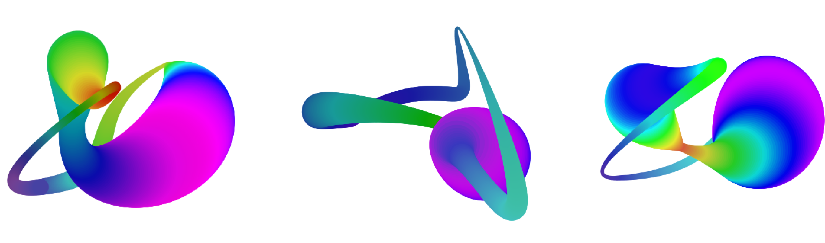
Here are some images that I made with this program, each drawn with the default of 500 dots.

If you want to play with this code, one place to start is by changing the way the curve is drawn. Rather than using a lot of overlapping dots, use a much smaller number of points on the curve, but draw short lines to connect each successive pair of points. Hint: use strokeWeight() to control the line thickness.

Here's the same idea but using Bezier curves instead. The only real change is to the type of the curve (from AUCurve to AUBezier ), and the routine newBezier() (which replaces newCurve() ). Making a smooth Bezier curve takes just a tiny bit more work because the control points have to be symmetrical around the knots.

import AULib.*;

int NumCurves = 2;      // The number of curves (not the number of knots)
AUBezier MyCurve;       // The curve itself
boolean Redraw = true;  // Only redraw when something changes

void setup() {
  size(500, 500);
  colorMode(HSB);  // everything in the sketch is in HSB
  newBezier();     // make a new curve
}

// draw the curve as a large number of equally-spaced dots
void draw() {
  if (!Redraw) return;  // don't bother redrawing the same thing
  background(255);      // white background
  noStroke();           // dots don't have an outline
  int numSteps = 500;   // how many dots to draw
  for (int i=0; i<numSteps; i++) {
    float t = norm(i, 0, numSteps-1);         // t runs from [0,1]
    float x = MyCurve.getX(t);                // get X at this t
    float y = MyCurve.getY(t);                // get Y at this t
    float diam = MyCurve.getIndexValue(t, 2); // get the diameter
    float hue = MyCurve.getIndexValue(t, 3);  // get the hue
    float sat = MyCurve.getIndexValue(t, 4);  // get the saturation
    float brt = MyCurve.getIndexValue(t, 5);  // get the brightness
    fill(hue, sat, brt);        // fill with this color
    ellipse(x, y, diam, diam);  // draw this dot
  }
  Redraw = false;    // don't draw again until something changes
}

// create a new AUBezier curve
void newBezier() {
  // each knot row: 0=x, 1=y, 2=weight, 3=hue, 4=saturation, 5=brightness
  float[][] knots = new float[1+(3*NumCurves)][6];  
  fillKnotWithRandom(knots, 0);    // handle knot 0 as a special case
  for (int i=0; i<NumCurves; i++) {
    int k = 1 + (3*i);
    if (k == 1) {
      // knot 1 is special because there's no knot -1 before 0
      fillKnotWithRandom(knots, 1); 
    } else {
      // knot k is symmetrical with knot k-2 around k-1
      for (int j=0; j<knots[0].length; j++) {
        knots[k][j] = knots[k-1][0] + (knots[k-1][j] - knots[k-2][j]);
      }
    }
    fillKnotWithRandom(knots, k+1);
    fillKnotWithRandom(knots, k+2);
  }
  /* Make the new curve. Give it the knots, tell it we have 2 
   * geometry values at the start of each row (the X and Y values),
   * and close it. Remember the geometry values must always come 
   * at the start of each row in the knots.
   */
  MyCurve = new AUBezier(knots, 2, true);   
  Redraw = true;    // we have a new curve, so draw it
}

void fillKnotWithRandom(float[][] knots, int whichKnot) {
  knots[whichKnot][0] = width * random(.2, .8);  // a value for X   
  knots[whichKnot][1] = height * random(.2, .8); // a value for Y not
  knots[whichKnot][2] = random(5, 50);           // line weight
  knots[whichKnot][3] = random(0, 255);          // hue 
  knots[whichKnot][4] = random(150, 255);        // saturation
  knots[whichKnot][5] = random(150, 255);        // brightness
}

void keyPressed() {
  switch (key) {
    case ' ':
      newBezier();  // make a new curve
      break;
    case '-':
      NumCurves = max(2, NumCurves--);  // use fewer curves
      newBezier();
      break;
    case '+':
      NumCurves++;   // use more curves
      newBezier();
      break;
    case 's':
      saveFrame();  // save the results to this directory
      break;
    case 'q':
      exit();       // quit!
      break;
  }
}

Here are some of the images. Note that because Bezier curves inherently have a lot more curviness to them, the diameter can drop below zero, which makes the circles disappear. To bring them back, increase the minimum diameter, or use the absolute value of the diameter by using abs(diam) rather than diam when drawing the circles.

A Constant-Length Tail

Here's an implementation of an example from earlier. We want to draw a little circle that's flying along a curve, leaving a trail behind. The trail is drawn of ever-smaller circles that are ever-more transparent.

The key thing is that the trail should always be the same length along the curve as the circle flies around. If you tried to write this using only Processing's built-in routines, it would be hard. But with the AU library, it's easy.

This little program makes a random big curve out of a bunch of Catmull-Rom segments, and then sends the circle flying around it. Its a fun animation to watch!

import AULib.*;

AUCurve MyCurve;           // the curve traveled by the ball
int NumTrailCircles = 100; // number of trails to draw
float TrailLength = .2;    // how much of [0,1] has the trail
float StartDiam = 30;      // diameter at start of trail
float RoundTripTime = 360; // number of frames for one trip

void setup() {
  size(500, 500);
  float[][] knots = new float[8][2];   // 8 knots usually looks good
  for (int i=0; i<knots.length; i++) {
    knots[i][0] = width * random(.2, .8);  // a value for X   
    knots[i][1] = height * random(.2, .8); // a value for Y 
  }
  MyCurve = new AUCurve(knots, 2, true);  // build the closed curve
}

// draw the trail from tail to head
void draw() {
  background(240, 210, 150);  // beige
  noStroke();
  float headT = frameCount/RoundTripTime;      // where we are now
  for (int i=0; i<NumTrailCircles; i++) {   // draw each circle
    float a = norm(i, NumTrailCircles-1, 0);   // a=1 at the tail, 0 at the head
    float distance = a * TrailLength;   // how far behind we are
    float trailT = headT + distance;    // t value here
    float x = MyCurve.getX(trailT);     // get the X for this element
    float y = MyCurve.getY(trailT);     // and the Y
    float opacity = 255 * a;            // opacity=1@head, 0@tail
    float diam = StartDiam * a;         // diameter drops to 0 at tail
    fill(165, 30, 30, opacity);         // fill with a shade of red
    ellipse(x, y, diam, diam);          // and draw this element
  }   
}

Here are some screenshots of the program in action.

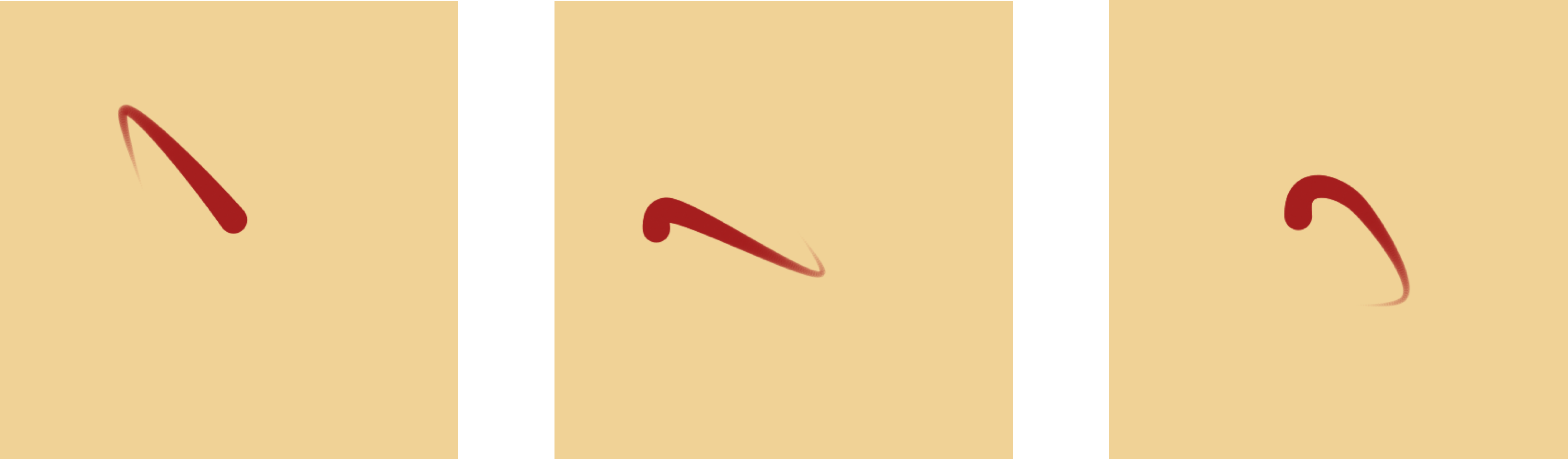
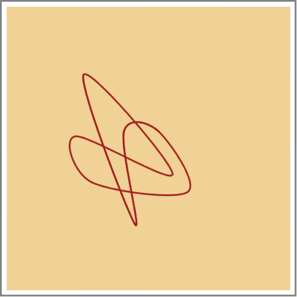
Just for fun, here's the curve that was used for the figures above. Note that becase the program uses random numbers, every run will produce a different curve.

Mixing your curves with AUBaseCurve

You might find it convenient sometimes to have a single array containing both Catmull-Rom curves and Bezier curves. Here's how.

Both AUCurve and AUBezier are subclasses of the type AUBaseCurve. In fact, the two subclasses contain nothing but their constructors, leaving all the work to the base type. So you can make an array of AUBaseCurve objects, and then freely send any of the methods in this document to any item in that array.

To help you keep track of what kind of curve you're holding, you can ask AUBaseCurve for the type of curve its got:

int getCurveType();  // returns CRCURVE or BEZCURVE

As noted in the comment, this returns one of two values:

• CRCURVE
• BEZCURVE

For example, you might create an array like this, where I'm assuming you've got a bunch of variables available that hold curve objects you've already made.

AUBaseCurve[] myCurves = { myBez1, myCR1, myCR2, myBez2 };

You could later use this array to draw dots along each curve. Notice that in the following code, I send getX() and getY() to objects of type AUBaseCurve , without worrying about whether they hold a Catmull-Rom or Bezier curve. To demonstrate how to use getCurveType() , I use the result of that call to set the fill color to red or green.

for (int i=0; i<myCurves.length; i++) {
  AUBaseCurve curve = myCurves[i];
  // CR curves are drawn with red dots, Bezier with green
  switch (curve.getCurveType()) {
    case AUBaseCurve.CRCURVE:  fill(255,0,0); break;
    case AUBaseCurve.BEZCURVE: fill(0,255,0); break;
   }

  int numSteps = 20;
  for (int step=0; step<numSteps; step++) {
    float t = norm(step, 0, numSteps-1);  
    float x = curve.getX(t);
    float y = curve.getY(t);
    ellipse(x, y, 10, 10);
  }
}

For technical reasons, you can only create AUBaseCurve objects by using the AUCurve and AUBezier constructors; you cannot create your own AUBaseCurve objects directly.

Tech Talk

Here is some information for advanced users.

Controlling Precision

When writing this library, I wanted query routines like getX() to run as quickly as possible. To make that happen, I precompute values for the curve's arc length at many points along the curve, and I save those values in a big table. When you query for data at a given t, I use binary subdivision in the table to quickly locate the proper interval, and then I use linear interpolate within that interval.

The downside of this is that it takes time to compute that table, and room to save it. The space isn't much of an issue for modern computers: as a rule of thumb, the number of samples I take for any given curve is roughly the arc length of the curve in pixels. This means that that your queries will generally be accurate to within a pixel.

But the time taken to compute this table might be an issue in some real-time programs. I need to compute this data when the curve is first created, and I need to re-compute it each time a knot is changed (actually, I just set a flag that re-computation is needed. The work doesn't happen until the next query, so you can make lots of changes in a row without the system constantly re-making the table after each one).

You can reduce the table-building time by reducing the size of the table. You adjust the size of the table (and thus the time required to produce it) by changing its density. Note that raising or lowering the density will have little effect on the speed of the query routines; you're just affecting the time and space required to build and save the table, and thus the accuracy of the query results. The density has a default value of 1. To adjust it, call

void setDensity(float density);
(default = 1)

This value is per-object, so different curves can have different densities. The library enforces a minimum density of .001. During computation of the table, it also enforces a minimum of 3 samples along each curve segment.

Note that lowering the density below 1 will cause the precision of your queries to degrade. Your returned points will always be on the curve, but as the density gets smaller the points will start to drift left and right from where they should be.

Increasing the density above 1 will increase the precision of the results, at the cost of a little more pre-processing time and a larger table.

Implementation Notes

The most convenient way to generate points on these curves is to use a matrix form, as nicely summarized by Tom Duff in his technical memo Families of Local Matrix Splines. Suppose we have a curve with knot values k0, k1, k2, and k3. Form them into row vector, which I'll call $\mathbf{k}$. We'll be using this in column form, so I'll use this vector in its transposed form, written $\mathbf{k}^T$. Now we want to find a point at the parameter value $t$ along the curve. I'll form a row vector $\mathbf{t}$ as $\mathbf{t} = [t^3 \;\; t^2 \;\; t \;\; 1]$.

To find the value of the curve at $t$, we need only one more thing: a 4-by-4 matrix, which I'll call $\mathbf{M}$. This matrix sits between the two vectors as in this tableau:

$$ \left[ \begin{matrix} t^3 & t^2 & t & 1 \end{matrix} \right] \left[ \begin{matrix} a & b & c & d \\ e & f & g & h \\ i & j & k & l \\ m & n & o & p \end{matrix} \right] \left[ \begin{matrix} k0 \\ k1 \\ k2 \\ k3 \end{matrix} \right] $$ Multiplied together, these three elements give us the scalar $\mathbf{t\;M\;k}^T$ , which is the value of the curve of matrix type $\mathbf{M}$ , with knot data $\mathbf{k}$ , at time $t$. Each particular kind of curve has its own characteristic matrix $\mathbf{M}$ that combines $\mathbf{t}$ with $\mathbf{k}$ in the just the right way. Both the cardinal splines (which include Catmull-Rom curves) and Bezier curves can be drawn with the same code, differing only in their own matrix.

The cardinal splines take a single parameter, which Duff calls $c$. When $c=0$ we get straight lines from knot to knot, and when $c=.5$ we get Catmull-Rom curves. Values of $c$ between those values blend between the polygon and Catmull-Rom forms. Values of $c$ outside that range produce very squiggly curves. Here is the cardinal matrix, and the Catmull-Rom matrix resulting from choosing $c=.5$.

$$ \begin{array}{lc} \mbox{Cardinal matrix:} & \left[ \begin{matrix} -c & 2-c & c-2 & c \\ 2c & c-3 & 3-2c & -c \\ -c & 0 & c & 0 \\ 0 & 1 & 0 & 0 \end{matrix} \right] \\ \\ \mbox{Catmull-Rom matrix:} & \left[ \begin{matrix} -.5 & 1.5 & -.5 & .5 \\ 1 & -2.5 & 2 & -.5 \\ -.5 & 0 & .5 & 0 \\ 0 & 1 & 0 & 0 \end{matrix} \right] \\ \end{array} $$

A nice derivation of the matrix form of the Bezier curve is described by Ken Joy in his note A Matrix Formulation of the Cubic Bezier Curve (note that Joy writes his ${\mathbf t}$ vector in the opposite order from the vector I'm using here, so I flipped his results to match. Here's the Bezier matrix ${\mathbf M}$:

$$ \begin{array}{lc} \mbox{Bezier matrix:} & \left[ \begin{matrix} -1 & 3 & -3 & 1 \\ 3 & -6 & 3 & 0 \\ -3 & 3 & 0 & 0 \\ 1 & 0 & 0 & 0 \end{matrix} \right] \\ \end{array} $$

To evaluate a 1D curve at $t$, we just put our knot values into $\mathbf{k}$, build $\mathbf{t}$, and evaluate $\mathbf{t\;M\;k}^T$. Because these curves are independent along each axis, we can blend as many values as we like for each value of $t$ just by changing $\mathbf{k}$. For example, to evaluate a 2D curve, with knot values for X and Y, we only need fill up $\mathbf{k}$. with the X values, and find $\mathbf{t\;M\;k}^T$. To find the Y value, just put the Y values into k $\mathbf{k}$ and again find $\mathbf{t\;M\;k}^T$. We can attach other data to each knot, such as stroke thickness or rainfall that day, and interpolate it as well.

This suggests that we can save some time, because we're only changing $\mathbf{k}$ from one query to the next. The product $\mathbf{t\;M}$ is the same for any data as long as $t$ doesn't change. And in fact that's just what I do. When you use any of the query routines to ask for a value, the system computes $\mathbf{t\;M}$ and saves it as a vector I'll call $\mathbf{a}$. It also saves the value of t that was used to build $\mathbf{t}$. Then it finds the appropriate data, loads the vector $\mathbf{k}$, and computes $\mathbf{a\;k}^T$. You can keep querying for other data at this value of t , and the library will keep re-using $\mathbf{a}$, saving you the cost of a vector-matrix multiply. When you query for a new value of $t$, it recomputes $\mathbf{a}$, saves the new value of t that was used, and proceeds as before.

We can use the same matrix to compute the derivatives, of course, and that's how I provide the tangent information. I cache $\mathbf{t}^\prime\mathbf{M}$ where $\mathbf{t}^\prime = [3t^2\;\;2t\;\;t\;\;0]$, and use it to compute the derivatives for any values of $\mathbf{k}$, only recomputing $\mathbf{t}^\prime\mathbf{M}$ when $t$ changes.

As I discussed in a blog post, you might think of saving some time by building a big table of pre-computed values of $\mathbf{a}$, for many different values of $t$. For any given $t$, you could find the closest such values, interpolate them, and have your $\mathbf{a}$. But if you count up the operations necessary to find and interpolate the values, its comparable to the matrix multiply, so this attempt at optimization doesn't pay off.

Resources

Thanks to Ginger Alford and Eric Haines for their help on how to structure the interface for this code, and comments on the documentation.

The library, examples, documentation, and download links are all at the Imaginary Institutes resources page:

https://www.imaginary-institute.com/resources.php

To use it in a sketch, remember to include the library in your program by putting

import AULib.*;

at the top of your code. You can put it there by choosing Sketch>Import Library... and then choosing Andrew's Utilities, or you can type it yourself.

This document describes only section of the AU library, which offers many other features. For an overview of the entire library, see Imaginary Institute Technical Note 3, The AU Library.