Table of Contents

• Introduction
• Overview
• Downloading and Using the AU Library
• Coin Flip
• Quick Blends
• Choosing
• Distances
• Easing
• Waves
• AUShuffle
• AUStepper
• AUField
• AUMultiField
• AUCamera
• AUCurve/AUBezier/AUBaseCurve
• Error Messages
• Consclusions

Introduction

This note summarizes the routines in version 1.0 of my AU (Andrew's Utilities) library for the Processing programming language.

The library consists of 12 distinct sections, each intended to help you with a different kind of task. Some sections contain a bunch of routines you can call directly, while others provide you an object which you first create, and then manipulate by calling its methods.

The ideas in this library were developed over the course of several years. Basically any time I found myself implementing something I'd implemented many times before, and which felt like a general-purpose idea to me, I bookmarked it in the back of my mind as something to put into a library one day. Recently I've been writing a lot of small Processing programs, and I've been writing the same code over and over. The time seemed ripe to finally put it all together.

This document is only meant to be a summary and reference. Detailed discussions for the major sections are available in a series of Imaginary Institute Technical Notes. Those sections that have a corresponding note will identify it at the start of the discussion. If such a note is mentioned, I strongly suggest you look it over. The notes were written to help you understand and use the library with efficiency and pleasure, and without stress. They also contain additional, detailed examples, along with important information and advice. The write-ups here are intended for use as a general overview, or later, as a quick refresher or place to look something up.

Also remember to check out the examples in the examples folder. There is a complete, ready-to-run program there for each section of the library, demonstrating its use. You can use these programs for experimenting, or even as a start for your own programs.

Here are the six notes that make up the AU library documentation:

• Imaginary Institute Tech Note 3: The AU Library
• Imaginary Institute Tech Note 4: Blending and Easing
• Imaginary Institute Tech Note 5: Waves
• Imaginary Institute Tech Note 6: Measuring Distances
• Imaginary Institute Tech Note 7: Fields and Cameras
• Imaginary Institute Tech Note 8: Equal Spacing Along Curves
• Imaginary Institute Tech Note 9: AU Library Quick Reference

Overview

There are 12 sections in the AU library. Here's a quick overview of each section. They're listed in the order in which they're discussed below. The sections that begin with AU describe an object that you create; the others are just collections of standalone functions.

Coin Flip

This is just a single routine. Half the time it returns true, the other half, false.

Quick Blends

It'ss often useful to smoothly blend between two values. You might be blending the position of an object over time, or its shape based on where it is on the screen, or even its color. A good-looking blend usually starts out and ends slowly, so that the endpoints aren't jarring. These routines offer fast and easy blends of this kind.

Choosing

Given a list of objects, select just one. You can attach weights to each object, which controls how likely it is that each object will be selected.

Distances

The conventional Euclidean distance is a great workhorse, but this section offers a bunch of other ways to measure the distance between two points. You can uses these to create unexpected geometry and images.

Easing

Easing is a general idea in animation that says that objects don't suddenly lurch into motion from a standing position, and they don't suddenly slam to a halt when they stop moving. Instead, objects need to pick up speed and then slow down. The easing sections offer you a variety of simple and complex ways to change values over time. They can also be used for non-animation purposes, of course.

Waves

This section provides you with a collection of repeating waves of different shapes. You can use them to create motion that repeats over time, or geometry that follows patterns on the screen.

AUShuffle

Given a list of objects, return them in randomized order. When they've all been returned, automatically shuffle the list again, so you can keep getting values.

AUStepper

Animations often happen in phases: do this, then do this, then do that. Within each phase, it's handy to know just how far along you've come. This section provides an object that lets you do handle this easily. You tell it how many phases you have and how long each one lasts. Then when you draw each frame, you ask it which step you're currently on, and where you are in that step. That makes it easy to draw the proper image.

AUField

We often want to manipulate 2D arrays of floats, whether to represent an image without being locked to just values from 0-255, or to represent some other information across the graphics window (or even just arbitrary 2D information). This object and its associated operations make it easy to work with this kind of data.

AUMultiField

An AUField, described above, are great for storing just one value per element, but what if we want to store and manipulate floats corresponding to a color image? This object packs multiple AUfield objects together, along with support routines. You can have as many fields as you like, but if you have at least 3, you can represent color images. There are many functions that work on any number of fields, but there are also a bunch that are designed specifically for treating 3 of the fields as RGB colors, or 4 of the as RGBA.

AUCamera

Motion blur is an important visual cue in many animations. This section makes it very easy to create and combine multiple images for each frame of animation to produce a nicely motion-blurred image. You can choose from a variety of shutter styles to get just the kind of motion blur you like. The AUCamera is meant for off-line rendering, when you can spend time producing each frame that will ultimately get assembled into a movie or animation.

AUCurve/AUBezier/AUBaseCurve

We often want to create equally-spaced points along multi-element Catmull-Rom and Bezier curves. These objects let you do do that easily. You can optionally close the curves automatically if you want, creating a smooth and continuous result. You can attach as many other floating-point values as you like to each knot, and they will be smoothly interpolated along with the geometric information in the knots.

Downloading and Using the AU Library

The AU Library can be downloaded from

https://www.imaginary-institute.com/resources.php

Install it in the usual way, following the instructions on processing.org for your type of computer and operating system. Once it's installed, include the library in your sketch by choosing Sketch>Import Library... and then choosing Andrew's Utilities. It will insert this line into your sketch (it should appear near the top):

import AULib.*;

Alternatively, you can type that in yourself.

To find out which version you'e using, call version() , which returns a String:

println("version = "+AULib.version());

There are three general things to know about using the library.

1. Some of the elements of the library (e.g., AUCamera) are objects that you create and manipulate. You make the object by calling its constructor, and then you ask it to do things for you by sending it messages. Some of these constructors want a pointer to your current sketch as the first argument (it's of type PApplet in the documentation below). With very rare exceptions, provide this argument with the keyword this .

2. Other elements (e.g. dist()) are just function calls that aren't associated with an object. To use them, just precede them with AULib:

if (AULib.flip()) println(heads);
            else println(tails);

3. Some routines make use of predefined constants, or choices. If the constant is associated with an object, precede it with the objects type, otherwise use AULib . For example, the distance function dist() is not part of any object, so its DIST_BOX element would be AULib.DIST_BOX , while one of the AUCamera shutter choices would be AUCamera.SHUTTER_OPEN .

Throughout the library, these predefined constants are integers. But no matter what, never use their numerical values rather than their names. The values assigned to these constants might change from one release of the library to the next, and if your code uses the old numbers, everything will go haywire. Always refer to these constants by name.

Coin Flip

This section contains just one tiny utility. It flips a fair coin and returns true half the time, and false the rest of the time. Really, this is just to save a little bit of typing, and to make some code just a tiny bit clearer:

boolean flip();

Here's a typical use:

float speedX = random(2, 4);  // move to the right
if (AULib.flip()) {
  speedX = -speedX;          // half the time, move left
}

Quick Blends

See Imaginary Institute Technical Note 4, Blending and Easing.

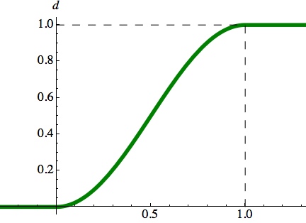
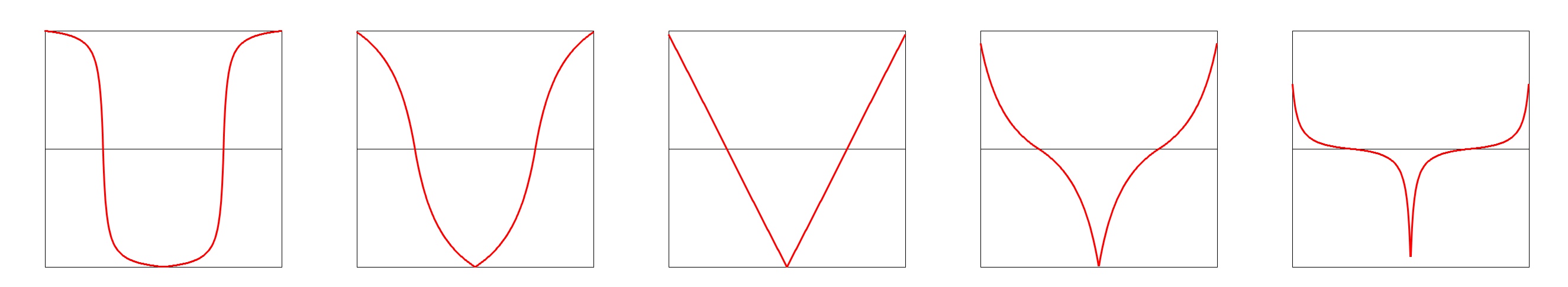
These are S-shaped blends: they start slow, pick up speed, slow down at the far end. The input is [0,1] and the output is [0,1]. They all have a derivative of 0 at both ends, so they start and stop smoothly. The first two versions produce results that are, practically speaking, identical, so I recommend using cubicEase() (or S() ) because it's faster. For more control over easing and blending, see the section on ease curves.

The first routine is based on a piece of the cosine curve:

// cosine-based blend 
float cosEase(float t);     

The next routine is based on an equation called a cubic:

// cubic-based blend
float cubicEase(float t); 
float S(float t);   

Finally, we have a variation on the cubic:

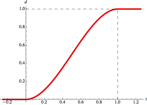
// quintic-based blend
float S5(float t);

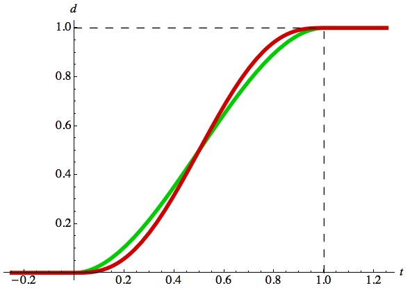
The S curve named S5() is a little flatter at the ends than the curves above. It's usually a subtle difference. Here is S5() in red, plotted over S3() in green (the name S5() comes from the nature of the equation that produces the curve).

Choosing

Sometimes you have a list of values and you want to choose just one of them. For example, you might have a program that draws a bunch of random balls moving around, but you've decided that even though everything about the balls is randomized, you like the way things look for just a few specific numbers of balls.

You can make an array of floats containing the values you like,

float[] ballCounts = { 7, 11, 13, 17, 19, 23, 29, 31, 37 };

and then get back one of these values:

float numberOfBalls = AULib.chooseOne(ballCounts);

chooseOne() considers each entry in the list to be equally likely to be selected. If you want some choices to be more likely than others, call chooseOneWeighted() with your list of values and a list of relative weights. The weights can be any values you like; they give the relative probabilities that the corresponding element in v will be returned. The number of weights must match the number of values. For example,

float[] values  = { 1, 2, 3 };
float[] weights = { 4, 3, 1 };
float myValue = AULib.chooseOneWeighted(values, weights);

will return the value 1 about half the time, the value 2 about 3/8 of the time, and the value 3 about one-eighth the time (note that these are probabilities over the long haul. Just as flipping a fair coin can quite possibly come up "heads" 50 times in a row, so too could you get the same value from this routine over and over. But flip that coin enough times, or call one of these routines enough times, and things will eventually approach their probabilities).

There's two versions of each routine: one for ints, and one for floats. Processing will pick the right one when you call it. You can also use an array of colors, because Processing saves those internally as ints. In both cases, the weights should be floats.

float chooseOne(float[] v);
int chooseOne(int[] v);
float chooseOneWeighted(float[] v, float[] w);
int chooseOneWeighted(int[] v, float[] w);

A common use of chooseOne() is to pick an element from an array. So if your array has N elements, you might make a list of integers with values { 0, 1, 2, , N-2, N-1 }, and then use that with chooseOne().

To make things easier for this common situation, you can hand chooseOne() just a single integer, and you'll get back a value from 0 to that integer minus 1:

int chooseOne(int n);

For example, all of these calls to chooseOne() produce the same results, applicable for use as an index into the values array defined on the first line:

int[] values = { 0, 1, 2, 3, 4, 5 };
// returns a value from the values array
int index1 = AULib.chooseOne(values);  
// returns a value [0, values.length-1]
int index2 = AULib.chooseOne(values.length); 
// returns a value [0, 5]
int index3 = AULib.chooseOne(6);  

You may notice that you could replace this final version of chooseOne() with a call to the built-in routine random() followed by a cast to an int. Using chooseOne() is no slower, and I think can be a little more clear in your code. Plus it offers you a little bit of easier flexibility down the line if you want to change the way you're choosing.

Distances

Imaginary Institute Technical Note 6, Measuring Distances.

The functions in this section are designed to help you find interesting distances between two points, A and P. The measurements involve a third point, B, which establishes a framework in which to make the measurement.

In all cases, when P=A, the distance returned is 0, and when P=B, the distance returned is 1. As P moves farther away from A, the distance increases without bound.

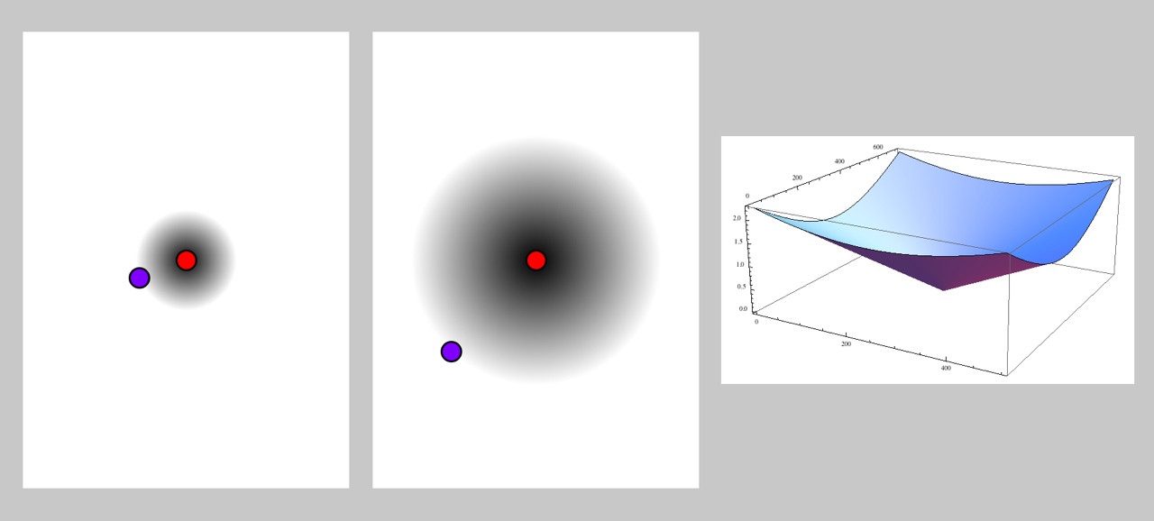
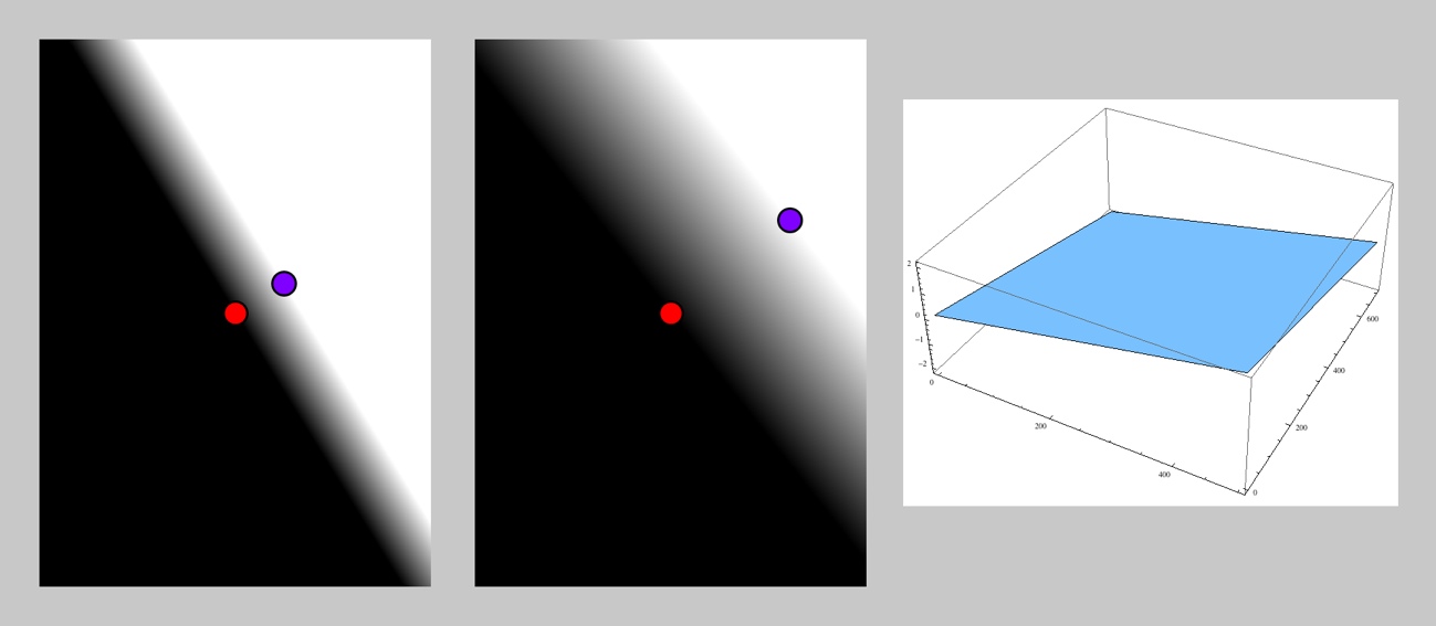
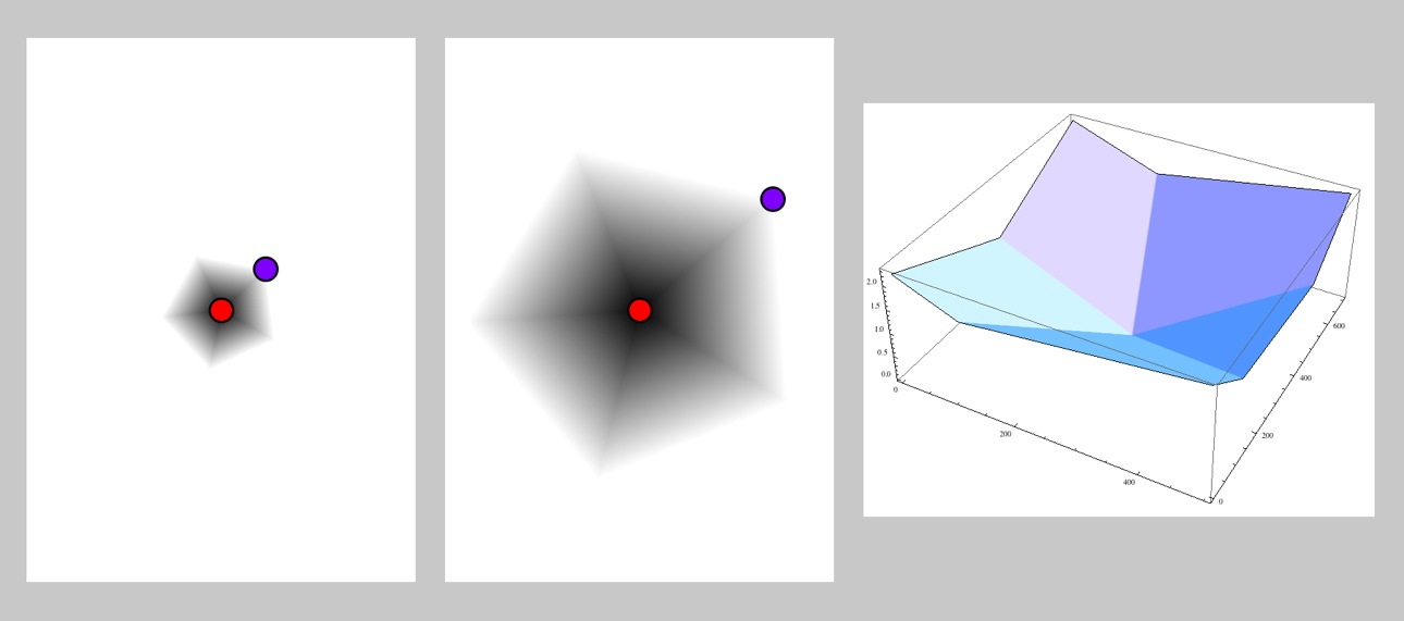
There are two distance routines. They both take the type of distance to be measured and the x,y values of points A, B, and P, and return a float representing the distance. The second call also takes an integer that further specifies the geometry. In the figures below, the red dot is A and the purple dot is B. A distance of 0 is black, and distances of 1 or more are white. For larger figures and more discussion, please see the technical note.

The first function is dist(), and can be found in AULib:

float dist(int distanceType, float ax, float ay, 
                             float bx, float by, 
                             float px, float py);

where

• ax, ay: coordinates of point A
• bx, by: coordinates of point B
• px, py: coordinates of point P
• distanceType: can take on any of the following five values (remember to precede these AULib. when you use them in a sketch):
  
  • DIST_RADIAL
  • DIST_LINEAR
  • DIST_BOX
  • DIST_PLUS
  • DIST_ANGLE

Here are each of the five choices, illustrated with a couple of vlaues for point B, and a plot showing the height of the distance function for a typical pair of values of A and B.

Radial Distance

The DIST_RADIAL type returns the standard Euclidean distance from A to B.

Linear Distance

The DIST_LINEAR type returns the distance from A to the point found by projecting P perpendicularly onto the line AB.

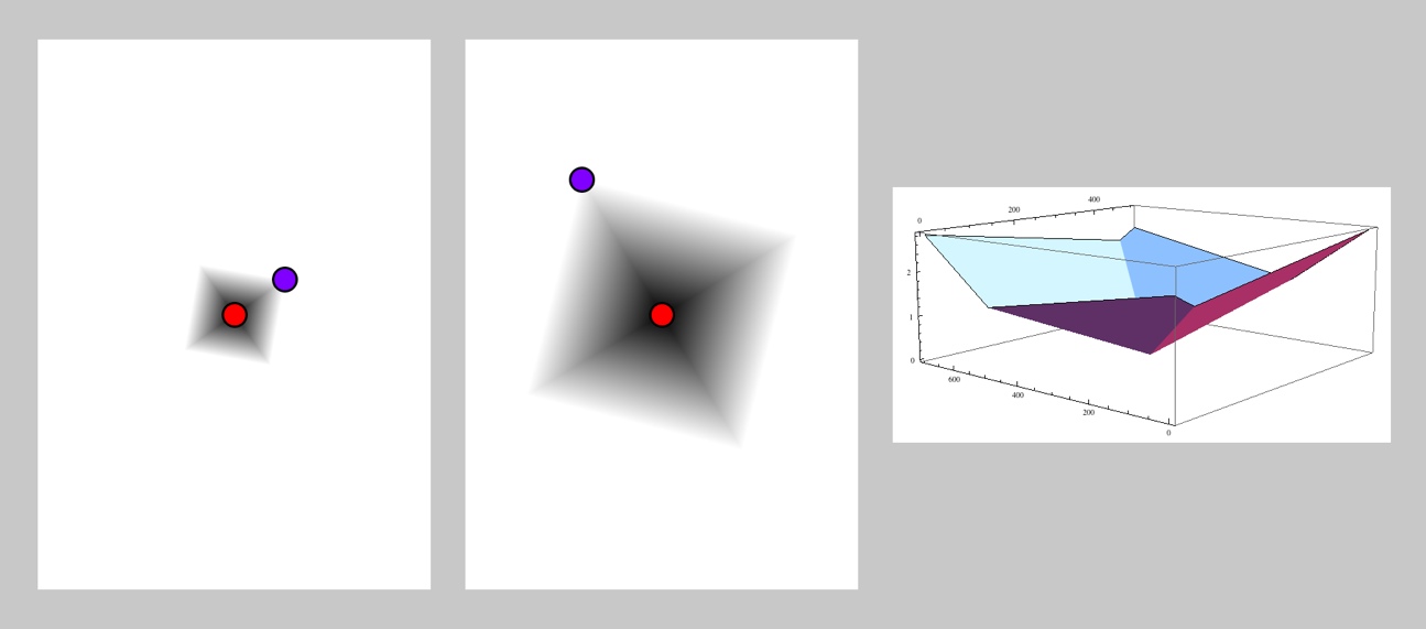
Box Distance

Using box distance, with type DIST_BOX, B is the corner of a box. Returns the distance from A to the projection of P on the line through the middle of the nearest side of the box.

Plus Distance

The plus distance, with type DIST_PLUS, is like linear distance, but also finds the distance from A to the point found by projecting P perpendicularly onto the perpendicular of AB, and returns the minimum of the two distances.

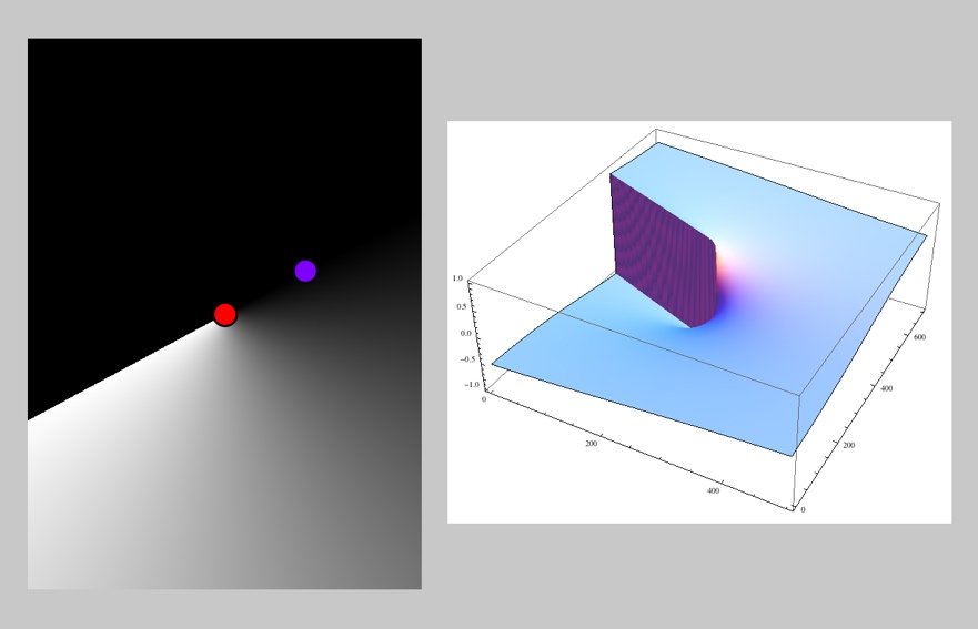
Angle Distance

Angle distance, with type DIST_ANGLE, finds the line from A to B, and measures the angle of the line from A to P clockwise from that first line.

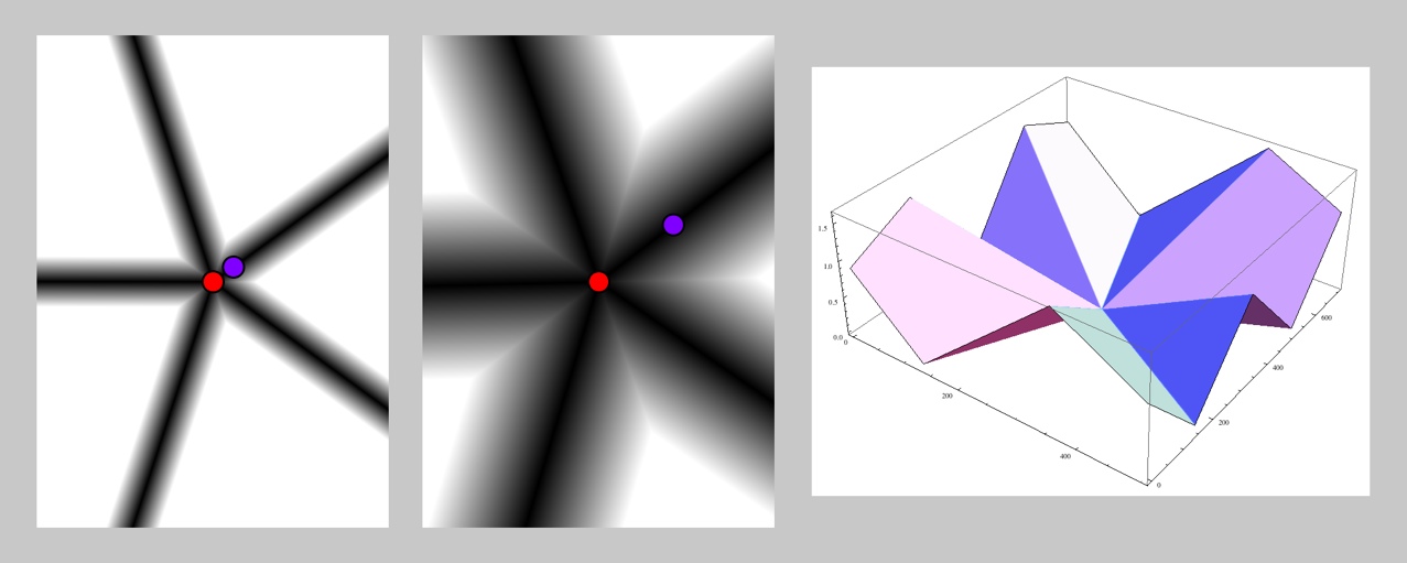
The second call takes one additional argument, which tells it how many sides are in the polygon that it uses to compute distances.

float distN(int distanceType, int n, float ax, float ay, 
                                     float bx, float by, 
                                     float px, float py);

where

• ax, ay: coordinates of point A
• bx, by: coordinates of point B
• px, py: coordinates of point P
• n: integer whose interpretation depends on distanceType
• distanceType: can take on the following two values (remember to precede these AULib. when you use them in a sketch):
  
  • DIST_NGON
  • DIST_STAR

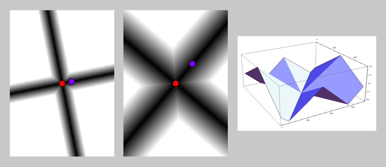
Here are the two cases, both illustrated for n=5.

Ngon Distance

Ngon distance, with type DIST_NGON, creates a regular n -sided polygon centered at A, with one vertex at B. Returns the smallest distance from P to any side of this polygon.

Star Distance

Star distance, with type DIST_STAR, creates a regular n -sided polygon centered at A, with one vertex at B, and draws a line from A through each vertex of this polygon. Projects P perpendicularly onto each of these lines, and returns the minimum of these distances.

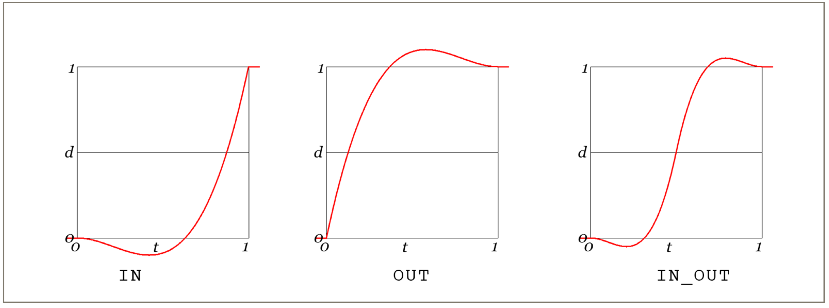
Easing

Imaginary Institute Technical Note 4, Blending and Easing.

These are ease curves. Each takes in a value of t from [0,1] and returns a value of 0 at t=0 and 1 at t=1. What happens in between varies for each curve. The technical note presents detailed information on each type of curve and practical advice for its use.

Theres just a single call for you to know:

float ease(int easeType, float t);

The value of easeType can take on any of these choices (remember to prefix each of these choice with AULib. in your code):

• EASE_LINEAR
• EASE_IN_CUBIC
• EASE_OUT_CUBIC
• EASE_IN_OUT_CUBIC
• EASE_IN_BACK
• EASE_OUT_BACK
• EASE_IN_OUT_BACK
• EASE_IN_ELASTIC
• EASE_OUT_ELASTIC
• EASE_IN_OUT_ELASTIC
• EASE_CUBIC_ELASTIC
• EASE_ANTICIPATE_CUBIC
• EASE_ANTICIPATE_ELASTIC

Linear

The output rises uniformly with t.

Cubic

The output follows a cubic curve.

Back

The curve gently undershoots and/or overshoots the enpoints.

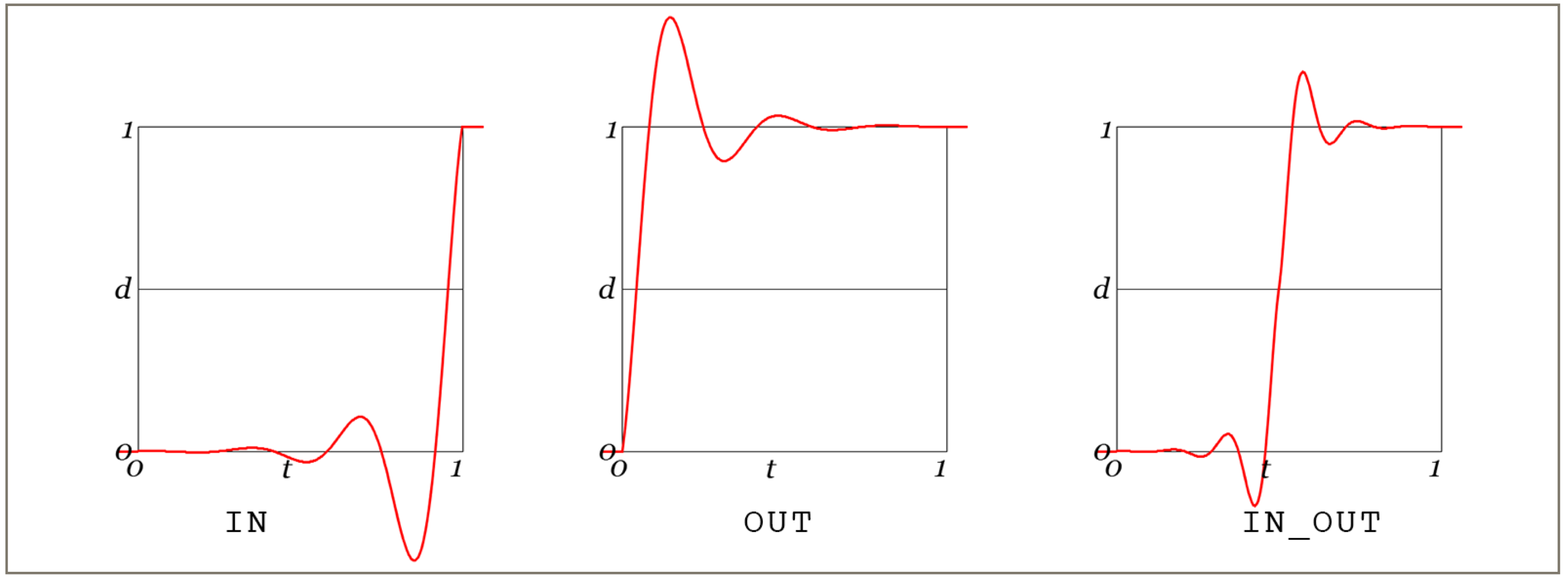
Elastic

The curve bounces at the start, finish, or both ends of the curve.

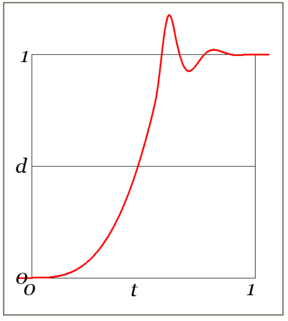
Cubic-Elastic

The output comes out of the start smoothly following a cubic, then bounces into the end.

Anticipate-Cubic

A short backwards anticipatory motion is followed by a smooth arrival at the end.

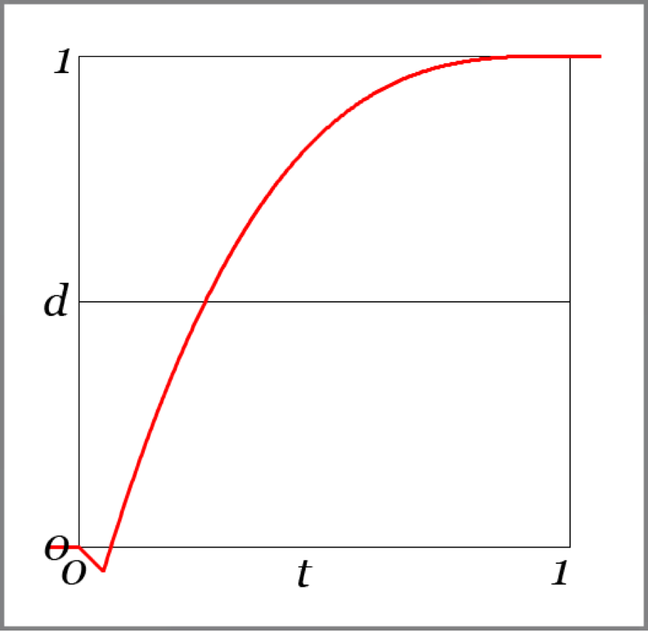
Anticipate-Elastic

A short backwards anticipatory motion is followed by a bounce into the finish.

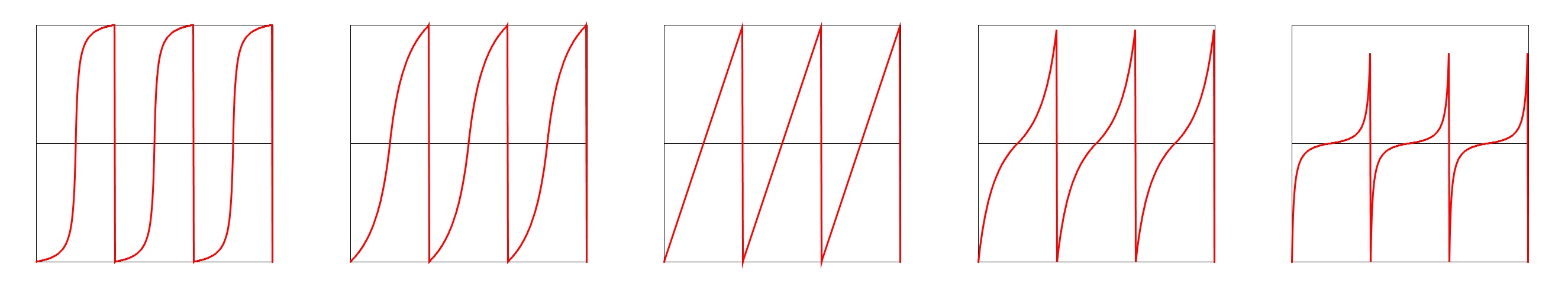
Waves

Imaginary Institute Technical Note 5, Waves.

The waves section provides you with repeating patterns of numbers. They're useful for creating anything that repeats, from cyclic animations to patterns in an image.

There is a single function:

float wave(int waveType, float t, float a);

The input waveType specifies which kind of wave you're interested in, selected from this list:

• WAVE_TRIANGLE
• WAVE_BOX
• WAVE_SAWTOOTH
• WAVE_SINE
• WAVE_COSINE
• WAVE_BLOB
• WAVE_VAR_BLOB
• WAVE_BIAS
• WAVE_GAIN
• WAVE_SYM_BLOB
• WAVE_SYM_VAR_BLOB
• WAVE_SYM_BIAS
• WAVE_SYM_GAIN

The value of t runs from 0 to 1, which spans one cycle of the wave. Values of t greater than 1 simply repeat the wave over and over. So t=1.25 produces the same result as t=.25, as does t=8.25 or even t=.75. The value a controls one parameter of the wave; just what a does depends on which wave you've chosen.

If you're using waves to control animation, it's common to use frameCount or millis() in an expression for t. For example, setting t to frameCount/60.0 will cause the wave to repeat every 60 frames indefinitely.

Most of the waves joint up smoothly as they repeat, others jump from their ending value to their starting value.

The values of waveType , and the effect of a , are described below. Much more information is available in the technical note. As always, don't forget to prefix each option with AULib. in your code.

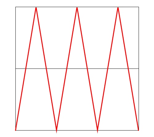
Triangle

The wave is symmetrical, rising from to 1 linearly and then back down. The value of a has no effect.

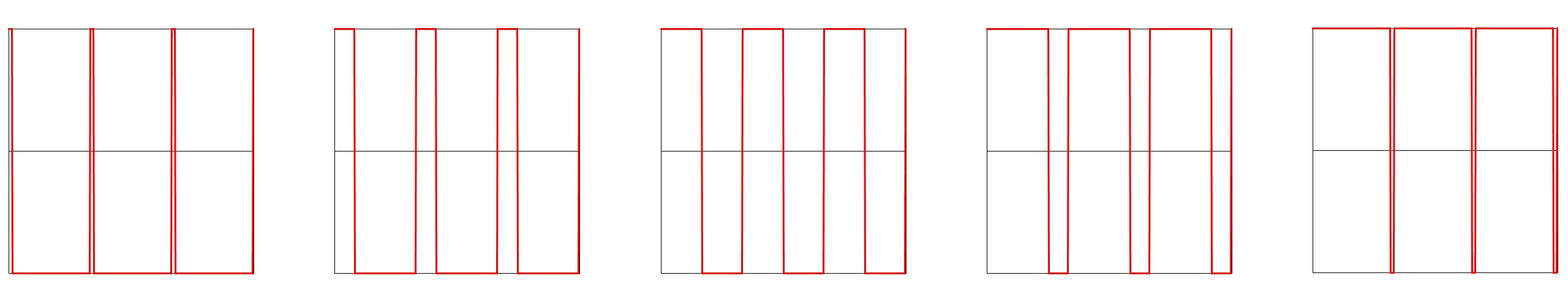
Box

The wave forms a box with height 1. The value of a controls the width of the box.

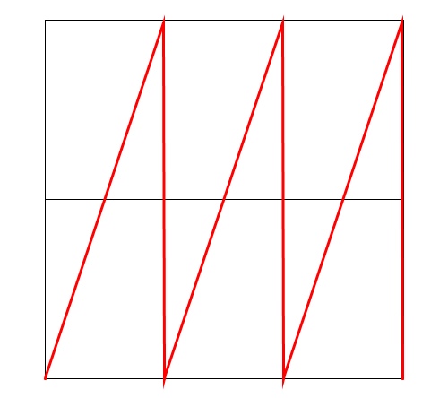
Sawtooth

A wedge-shaped wave that rises from 0 to 1. The value of a has no effect.

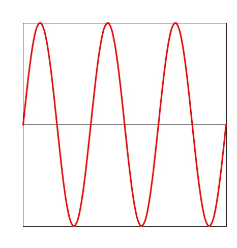
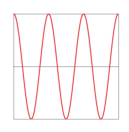
Sine

This is a sine wave. The value of a controls how much of the wave gets used in the interval from t=0 to t=1. Specifically, the output is sin(2 pi a t).

Cosine

This is a cosine wave. The value of a controls how much of the wave gets used in the interval from t=0 to t=1. Specifically, the output is cos(2 pi a t).

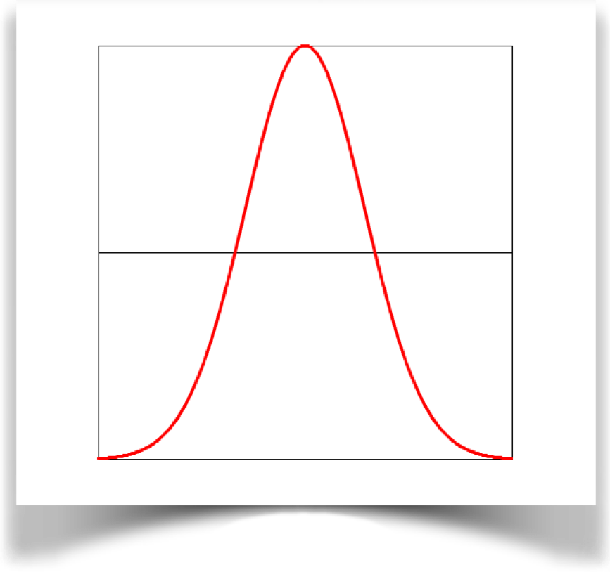
Blob

This is the right half of a Gaussian curve. The parameter a has no effect.

Variable Blob

This is the right half of a Gaussian, but you can control the width of its central peak. When a=0 you get a regular Gaussian as above, and when a=1 you get something much more narrow.

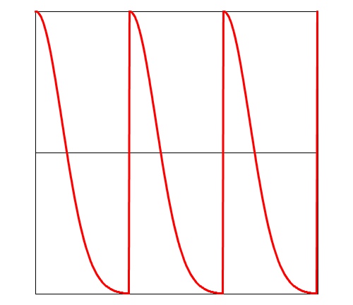
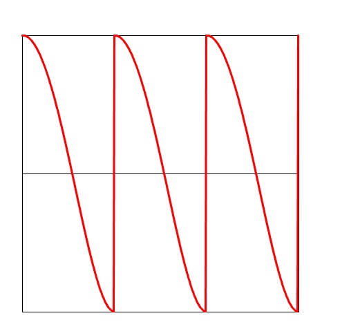
Bias

This curve pulls into one of the corners. When a=0 it pulls in the lower-right, so it starts slowly and then finishes fast. As a=.5 increases, the line straightens out, until when a=.5 it's just like a linear wave. As a gets larger, the curve pulls into the upper-left corner, starting fast and ending slower. This behavior is at its most pronounced when a=1.

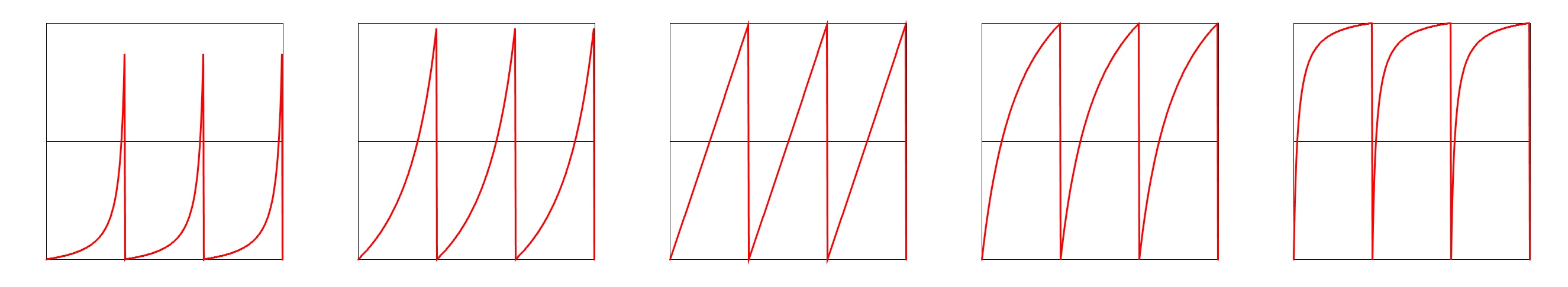
Gain

This curve combines the Bias curve above with an S curve. Think of a scaled version of the bias curve forming the first half, and its reflection forming the second half. The value of a controls the shape, just as for the bias curve.

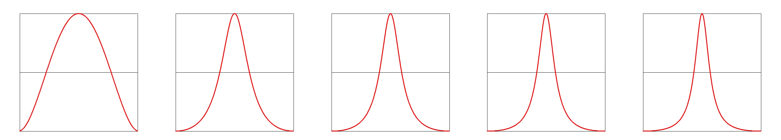
Symmetrical Blob

This is a symmetrical version of the blob curve. The parameter a has no effect.

Symmetrical Variable Blob

This is a symmetrical version of the blob curve. The parameter a has the same effect as for the regular value of the WAVE_VAR_BLOB curve. Thus if you want to make a symmetrical, traditional Gaussian, use this curve with value of a=0.

Symmetrical Bias

This is a symmetrical version of the bias curve. The parameter a has the same effect as for the regular value of the WAVE_BIAS curve.

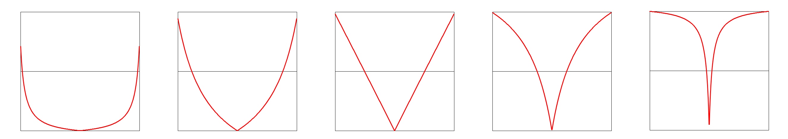
Symmetrical Variable Gain

This is a symmetrical version of the gain curve. The parameter a has the same effect as for the regular value of the WAVE_GAIN curve.

AUShuffle

Think of playing a game with cards. You shuffle the deck, and then deal the cards one by one, so you're getting them in random order. You get each card only once until the deck is exhausted. Then you gather up all the cards, shuffle the deck again, and keep dealing.

This is a very useful kind of operation in programming. A common example is to create a list of colors that you want to use over and over. Another example is when you use a variety of shapes that you want to draw with over and over. In both cases, you want to use up all the items in your list before you repeat any of them.

The AUShuffle object was designed for just this. To create one, hand it an array of floats. Then call next() to get back one of the floats. The library will return a random entry from your list, and then another and another, until theyve all been returned once. Then it re-shuffles your original list and starts over.

A nice feature of the AUShuffle object is that when it makes sure that the first object returned from the new list is different from the last object returned from the old list. That way you'll never get the same value twice in a row, even after a shuffle.

AUShuffle(float[] v);
float next();

What if you want to use a list of some other type, such as ints or even your own custom types of objects? The easy way is to make a list of the indices of your array. For example, if you have 10 objects that you want to shuffle, make a list of floats with the values 0 through 10, and make an AUShuffle object. Each time you call next() , you'll get back an index from your list, which corresponds to an object in your array. Because next() returns a float, and a float can have a tiny bit of noise in its value, I recommend passing the results through Processing's round() routine to make sure you're using the integer you wanted. Here's an example for filling up a basket with a few hundred Egg objects drawn from an array with only six of them.

void scrambleEggs() {
   // assume global variables for our six egg objects
   Egg[] myEggs = { Egg0, Egg1, Egg2, Egg3, Egg4, Egg5 };
   float[] indices = { 0, 1, 2, 3, 4, 5 };
   AUShuffle shuffler = new AUShuffle(indices);
   for (int i=0; i<500; i++) {
      Egg thisEgg = myEggs[round(shuffler.next())];
      thisEgg.includeInBasket();
   }
}

Using AUShuffle to select elements from an array is common enough that there's a shortcut. Rather than creating an array with the indices 0 through the array length minus 1, as in the above example, you can just call AUShuffle with a single index. It will presume that's the array length, and calls to next() will return values from 0 to that length minus 1:

AUShuffle(int n);

Here's the code above, but using this version. The big change is that line 4 from the first listing has disappeared: we no longer have to make the array called indices:

void scrambleEggs() {
   // assume global variables for our six egg objects
   Egg[] myEggs = { Egg0, Egg1, Egg2, Egg3, Egg4, Egg5 };
   AUShuffle shuffler = new AUShuffle(myEggs.length);
   for (int i=0; i<500; i++) {
      Egg thisEgg = myEggs[round(shuffler.next())];
      thisEgg.includeInBasket();
   }
}

AUStepper

Many animations, even short ones, involve several phases, or steps. You might have separate routines for drawing each step (for example, step 1 shows a growing square, step 2 rotates the square, and step 3 shrinks it back down). Each of these routines takes a value from 0 to 1, giving it the normalized location along that step, and it draws the corresponding picture.

These phases rarely have the same length, so using frameCount or millis() to find out which step you're in, and where you are in the step, can take some work. The AUStepper is designed to do that work for you.

First declare a global object of type AUStepper , but don't create it yet. You'll actually make it in your sketch's setup() by calling one of the three constructors.

The first constructor takes an integer and an array of floats. The integer tells the controller how many frames long your animation will be. The array of floats tells it the relative length of each step. The float array doesn't have to add up to 1, or anything else, because the values are all relative. For example, if you hand it an array with the values { 3, 6.5, 9.25, 7 } then you're telling it you have four steps with those relative lengths. The controller figures out how many frames to assign to each step based on the total length of the animation.

The second constructor takes an array of ints, one for each phase. This tells the controller explicitly the length in frames of each phase.

The third constructor is a convenience for those times when all your steps take the same number of frames. It takes an int telling it how many steps you want, and another int telling it how many steps are in each frame.

Whichever constructor you choose, the next steps are the same. In your draw() routine, call the step() method on your controller, and then save the values you get by sending getStepNum() and getAlfa() to the controller (I spell the word alpha phonetically because alpha is a reserved word in Processing) These tell you which step number you're on right now (starting at 0), and where you are in that step (running from 0 to 1). In our example, we have 4 steps, so over the course of the animation, stepNum will run from 0 to 3. For each value of stepNum , alfa always starts at 0 and ends one step short of 1.

That's all you need to do for basic animation.

Theres an optional step that is sometimes very useful. Normally alfa eases in and out of every step using a cubic S-curve (see Section 6, Quick Blends). You may not want that behavior. For example, if something is moving across the screen, you may want it to move at constant speed, and not speed up and slow down at the start and end of each step.

You can tell the controller which kind of easing to use independently for each step. For each step, you provide an integer corresponding to one of the EASE types (see Section 9, Easing). If you want different eases for each step, you can make an array of these values and hand that array to setEases() . If the array isn't as long as the number of steps, the system just keeps re-using the list from the start. If you don't want any easing for a given step, then specify EASE_LINEAR for that step. If you want to set the same ease type for all your steps, call setAllEases() with that type.

The value you get back from getAlfa() goes from 0 to 1 over the course of each phase. So if you have three phases in your animation, first stepNum will have the value 0 as alfa goes from 0 to 1, then stepNum will have the value 1 as alfa again goes from 0 to 1, and finally stepNum will be 2 as alfa yet again goes from 0 to 1. If youd rather have a single value that runs from 0 to 1 over the course of the entire animation, call getFullAlfa() .

If you're using an AUCamera object, read the section on Coordinating an AUStepper and an AUCamera in Section 15 ( AUCamera ) for some useful advice. In particular, the AUStepper routine getFullAlfa() returns the same value as the AUCamera routine getTime() .

Here's a summary of how to set up and use an AUStepper :

Step 1, declare a global

You'll want to declare a global object of type AUStepper so that you can use it throughout your sketch. Just declare it here. We'll initialize it in the next step.

AUStepper Stepper;  // declare a global Stepper

Step 2, in setup(), create your controller

Once you're inside of , you can create the controller. There are three different ways to create the controller.

1. Option 1: give relative lengths and a total frame count.

   float[] stepLengths = { 1, .5, .5 }; // can be of any length
   float numFrames = 50;                // length of animation
   Stepper = new AUStepper(numFrames, stepLengths); 
   

2. Option 2: explicitly give the length in frames of each phase.

   int[] frameCounts = { 100, 150, 175 }; // can be any length
   Stepper = new AUStepper(frameCounts);
   

3. Option 3: give number of steps and frames per step.

   Stepper = new AUStepper(3, 60); // 3 steps, each 60 frames long
   

Step 3, use your controller in draw()

Use your global AUStepper object to find the current step number, and where you are in that step. Then you'll often jump to a little routine for drawing images corresponding to that step, passing it the value of alfa so it can the picture corresponding to that percentage along the step.

Stepper.step();
float alfa = Stepper.alfa();
switch (stepNum) {
   case 0: drawStep0(alfa); break;
   case 1: drawStep1(alfa); break;
   case 2: drawStep2(alfa); break;
}

Optional: Set the easing in each step.

Typically this will come right after creating the controller in setup():

int[] easeTypes = { // list gets re-used if too short
   AULib.EASE_IN_OUT_CUBIC, 
   AULib.EASE_OUT_BACK,
   AULib.EASE_IN_OUT_ELASTIC };   
Stepper.setEases(easeTypes);

or to set them all at once,

Stepper.setAllEases(AULib.EASE_IN_OUT_BACK);

AUField

Imaginary Institute Technical Note 7, Fields and Cameras.

When working with images, it's often very helpful to be able to hold a value for every pixel. If that value is a color, then of course we can use the on-screen graphics window itself, or an off-screen PGraphics object. But if we need the range and precision of a float, we have to roll our own data structure.

An AUField is just a 2D array of floats, with a bunch of useful routines already created for them. Unlike many objects, the internal data of an AUField is very much meant for you to get into, read, and write. The existing routines are there to save you the trouble of writing your own for many common tasks.

Inside an AUField there are three variables:

• int w: the width of the field. Never assign a new value to this!
• int h: the height of the field. Never assign a new value to this!
• float[][] z: the 2D data. As usual, access this by z[y][x] for the element (x,y)

Note that the first two fields, w and h, are integers that you can read and write. Dont write to w and h!

I could have hidden them behind routines that returned them, but they're so frequently useful and they pop up so much in loops that I didnt want to make you go through the time and hassle of calling something like getW() over and over. So I'm giving you great power here, and you need to use great responsibility. The contents of the 2D array named z are yours to read and write as you like, and you can read w and h all you want, but never write new values into w and h. If you want to change the size of your field, create a new AUField object!

Creating

To create a field, you hand a pointer to your sketch, followed by your desired width and height:

AUField myField = new AUField(PApplet app, int wid, int hgt);

With very rare exception, the first argument should simply be the keyword this, which tells the new AUField how to talk to you your sketch. The z array in the field will be created with your specified width and height, which typically will be the same width and height as your graphics window. Your new field starts out with a value of 0 at every location.

Reading and Writing

Here's the call to fill up an AUField from the current graphics windows pixels:

void fromPixels(int valueType);

When copying pixels to an AUField, you need to decide how the RGB data in each pixel should be converted into a single float appropriate for the field. You express your choice by choosing a value for valueType. Your choices are:

• FIELD_RED: Save just the red value.
• FIELD_GREEN Save just the green value.
• FIELD_BLUE Save just the blue value.
• FIELD_AVG_RGB: Save the average of red, green, and blue
• FIELD_LUM: Save the luminance (.3*red + .59*green + .11*blue)

If your pixels are in shades of gray, then these will all return the save value. In that case I suggest using any of the colors (e.g., FIELD_RED ) as they are a tiny bit faster than the average and luminance options.

To draw your field on the screen, just tell it where to put the upper-left corner:

void toPixels(int dx, int dy);

Here each field entry becomes a gray pixel, so you'll probably want your pixels to have values between 0 and 255. Anything below 0 will be black, and anything above 255 will be white.

You can also pass your drawing through another field which acts as a mask. On a pixel-by-pixel basis the mask blends your fields color (a shade of gray) with the screen pixels existing color. A black pixel in the mask (value 0) means the field contributes nothing, while a white pixel in the mask (value 255) means the field color completely replaces the pixel color. Values between 0 and 255 produce blends of the two colors.

void toPixels(float dx, float dy, AUField mask);

The mask by default is placed so its upper-left corner is on the upper-left corner of the picture. You can shift the upper-left corner of the mask relative to the upper-left corner of the picture.

void toPixels(float dx, float dy, AUField mask, float mx, float my);

You can write your field into an offscreen PGraphics object instead of the onscreen pixels, if you want. It should be the same size as your field. These calls do the job:

void toPixels(float dx, float dy, PGraphics pg);
void toPixels(float dx, float dy, AUField mask, PGraphics pg);
void toPixels(float dx, float dy, AUField mask, float mx, float my, PGraphics pg);

Note that for efficiency reasons, toPixel() ignores any transformation commands you may have issued (like translate(), rotate(), or scale()). To draw your picture so that these transformations have effect, write it to a PGraphics object, and then draw the resulting PGraphics object with image(). You can see demonstrations of this technique in the example programs.

Flattening

To assign a single value to every entry in the field, call

void flatten(float v);

Scaling the Range

You'll often want to scale your data so that it fills a certain range. Probably the most common example of this is to scale everything to (0, 255) so that you can display it:

void setRange(float zmin, float zmax);

If you want to scale to the range (0,1), there's a shortcut to save you some typing:

void normalize();

Arithmetic

You can add a fixed value to every entry in the field:

void add(float a);

You can multiply every entry in the field by a given value:

void mul(float a);

You can also combine two fields by adding or multiplying them element by element:

void add(AUField f);
void mul(AUField f);

Copies and Duplicates

You can copy one field to another, as long as they're of the same size:

void copy(AUField destination);

You can also create a brand-new, independent duplicate, or dupe, of any field:

AUField dupe();

Example Use of AUField

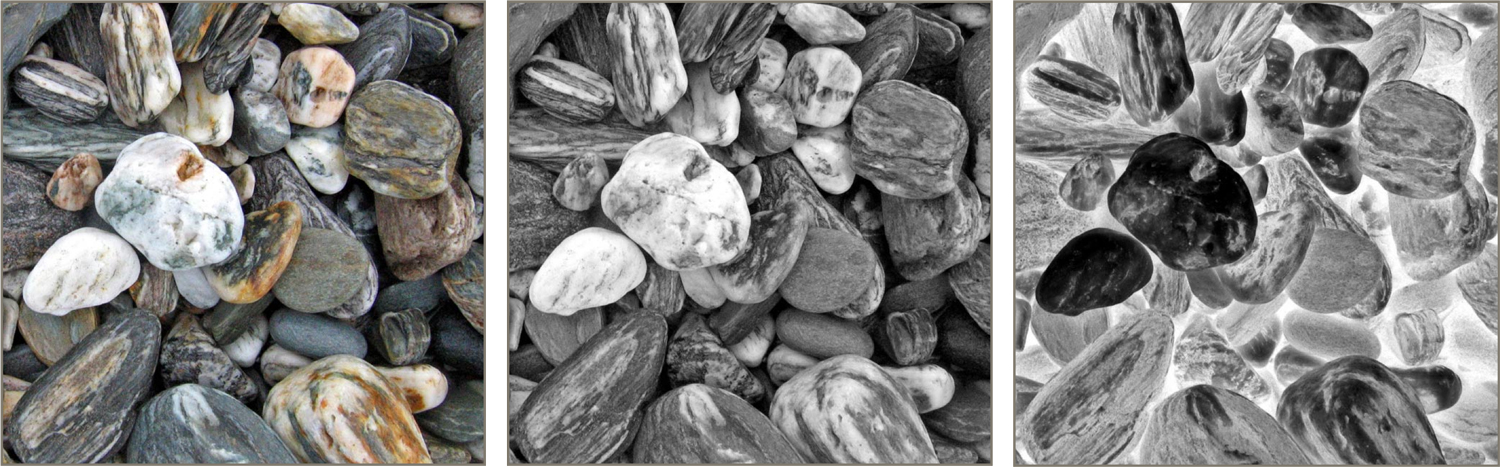
Let's use a field to make the negative of a photograph. Here's the code (its so short, we don't even need a draw() routine):

void setup() {
 PImage Img = loadImage("BeachRocks.jpg");
 size(Img.width, Img.height);
 image(Img, 0, 0);
 saveFrame("first.tif"); // save the starting image
 int numGrays = 4;
 AUField field = new AUField(this, width, height);
 field.fromPixels(AUField.FIELD_LUM);
 field.toPixels(0, 0);
 saveFrame("bw.tif");   // save the lum version
 for (int y=0; y<field.h; y++) {
   for (int x=0; x<field.w; x++) {
     float v = field.z[y][x];  // get the value at (x,y)
     field.z[y][x] = 255-v;    // replace it with the inverse
   }
 }
 field.toPixels(0, 0);     // copy the field to the screen
 saveFrame("inverse.tif"); // and save it
}

Here are the results:

AUMultiField

Imaginary Institute Technical Note 7, Fields and Cameras.

An AUField is fine for a grayscale image, but color pictures typically have three channels , one each for red, green, and blue. Of course, you can represent and work with a color picture by creating three fields, one for each channel. That's where the AUMultiField comes in. An AUMultiField is very similar to an AUField , with just a few changes to accommodate the fact that the data is now held in an array of fields, rather than just one. If you happen to choose 3 or more fields, you can treat those as red, green, and blue values for pixels. I'll go through these pretty fast, assuming you're already familiar with the AUField methods discussed in Section 13, AUField .

Creating

To create an AUMultiField , you give the constructor a pointer to your sketch (using the keyword this ), followed by the number of fields, you want it to hold (at least three for RGB images), followed by integers stating your desired width and height:

AUMultiField myField = new AUMultiField(PApplet app, int numFields, int wid, int hgt);

Your new AUMultiField starts out with a value of 0 in every position of every field.

Like an AUField , you can reach in and mess with the data. Here are the internal fields:

• int w: the width of the field. Never assign a new value to this!
• int h: the height of the field. Never assign a new value to this!
• AUField[] fields: an array of AUField objects (change the contents of these fields all you like)

Like with the AUField, I'm giving you read and write access to w and h to save you some time and typing. You can read these, but never write new values into w and h!

The fields object contains one AUField for each color channel. They all have the same width and height.

If you're storing colors, the first three elements in the fields array will contain red, then green, then blue. So for example, the green value at entry x=2, y=6 is written this way:

myField.fields[1].z[6][2]

where I'm specifying field 1 (that's the second, or green, field) at location y=6 and x=2.

Reading and Writing

You can fill up the first 3 or 4 fields of your AUMultiField objects with RGB or RGBA values from the screen pixels.

void RGBfromPixels();
void RGBAfromPixels();

You can write to the screen, either writing opaque RGB values from fields 0, 1, and 2, or writing RGBA values from the first 4 fields.

void RGBtoPixels(float dx, float dy);
void RGBAtoPixels(float dx, float dy);

If youd rather use an external mask rather than a built-in alpha field, you can. As with an AUField mask, you can optionally offset the mask in x and y before applying it.

void RGBtoPixels(float dx, float dy, AUField mask);
void RGBtoPixels(float dx, float dy, AUField mask, float mx, float my);

As with an AUField , there are versions of each of these calls for writing into a PGraphics object, rather than the screen:

void RGBfromPixels(PGraphics pg)
void RGBAfromPixels(PGraphics pg)
void RGBtoPixels(float dx, float dy, PGraphics pg);
void RGBAtoPixels(float dx, float dy, PGraphics pg);
void RGBtoPixels(float dx, float dy, AUField mask, PGraphics pg);
void RGBtoPixels(float dx, float dy, AUField mask, float mx, float my, PGraphics pg);

Technical note for graphics people: all of the routines in the AU library work with color values that have not been pre-multiplied by alpha (that's how Processing does it, so to prevent confusion and problems, that's how I do it, too).

Flattening

If you have at least 3 fields, you can treat the first 3 as colors and set them all at once:. You can assign the same value to every RGB or RGBA entry in every field:

void flattenRGB(float fr, float fg, float fb); 
void flattenRGBA(float fr, float fg, float fb, float fa);

You can set all the pixels of all the fields in your AUMultiField at once to the same value:

void flatten(float v);

You can just set all the pixels of any specific field to the same value:

void flattenField(int fieldNumber, float v);

Setting and Getting Multiple Values

You will usually assign values directly into the fields array. There are conveniences for setting the first three or four fields at once:

void setTriple(int x, int y, float v0, float v1, float v2);
void setQuad(int x, int y, float v0, float v1, float v2, float v3);

If you're using your AUMultiField to store colors (either RGB in the first three fields, or RGBA in the first four), there are some convenience routines to save you some time and effort when converting to and from Processing's color type.

You can set the first three fields with RGB values, or the first four with RGBA values, with

void RGBAsetColor(int x, int y, color c);
void RGBsetColor(int x, int y, color c);

Going the other way, you can get back a color if you have at least 3 (or 4) planes:

color getRGBAColor(int x, int y);
color getRGBColor(int x, int y);

Scaling the Range

You can scale your color image in two ways.

Scaling separate means that each color channel is individually scaled. That is, the library finds the minimum and maximum red values, and then scales all the red values to fill the range you've provided. Then it does the same thing for green, and then blue. This ensures that each color channel fills the entire range, but it can change the composite colors you see on the screen, because the RGB values are usually not being scaled by the same amount. This can be useful when you're working with abstract data, but if your data is a picture of some kind, it can make it look weird.

Scaling together means the library finds the smallest and largest values in all the channels at once, and then scales all three channels by those same values into your range. Thus you're guaranteed that at least one color in at least one pixel will have the largest value you specify, and and at least one color in at least one pixel will have the smallest value you specify. If you're manipulating color images, this is usually the choice you want.

There are two calls for each type of range-setting. If you want to scale all the fields in your object, use these:

void setRangeTogether(float zmin, float zmax);
void setRangeSeparate(float zmin, float zmax);

If instead you want to only affect the first few fields, these variations will only work with fields numbered 0 to numFields, leaving the rest alone:

void setRangeTogether(float zmin, float zmax, int numFields);
void setRangeSeparate(float zmin, float zmax, int numFields);

Frequently we want our new scale to be [0,1]. To save you a little typing, there are shortcuts for that. These correspond to the four calls above, but merely set zmin to 0 and zmax to 1 for you:

void normalizeTogether(int numFields);
void normalizeSeparate(int numFields);
void normalizeTogether();
void normalizeSeparate();

Similarly, when working with colors we often our new scale to be [0,255]. These calls scale the first three fields to [0,255]:

void normalizeRGBTogether();
void normalizeRGBSeparate();

And these scale the first four fields to [0,255]:

void normalizeRGBATogether();
void normalizeRGBASeparate();

Arithmetic

You can add a fixed value to every entry in every field:

void add(float val);

You can multiply every entry in every field by a given value:

void mul(float val);

As usual, there are shortcuts if you have at least 3 fields to store RGB values:

void RGBadd(float fr, float fg, float fb);
void RGBmul(float mr, float mg, float mb);

Or if you have at least 4 fields to store RGBA values:

void RGBAadd(float fr, float fg, float fb, float fa);
void RGBAmul(float mr, float mg, float mb, float ma);

As with AUField objects, you can also combine one AUMultiField with another by adding or multiplying them element by element:

void add(AUMultiField mf);
void mul(AUMultiField mf);

Copies and Duplicates

You can copy one AUMultiField to another, as long as they're of the same size. To copy your AUMultiField into a destination, hand that target to your original:

void copy(AUMultiField dst)

You can also create an independent duplicate, or dupe, of any AUMultiField:

AUMultiField dupe();

Copying and Swapping Layers

You can easily copy one field to another with

void copyFieldToField(int from, int to);

If you want to copy several successive fields at once, use

void copySeveralFields(int from, int to, int n);

This will copy field from to field to , then ( from+1 ) to ( to+1 ), and so on, n times. The two ranges can overlap.

Similar routines exist for swapping either one or several fields:

void swapFields(int a, int b);
void swapSeveralFields(int a, int b, int n);

Composition

You can compose one color AUMultiField over another using the standard Porter-Duff over operator (as always, all work is done with non-pre-multiplied color values):

void over(AUMultiField B);

This will compose the calling field over B, and modify B to hold the result. If B has only three fields it will be presumed to have an alpha value of 1 everywhere. If B has a fourth field, that field will be used for B s alpha, and will be updated properly.

If you provide a mask, that will be used for the calling fields alpha:

void over(AUMultiField B, AUField mask);

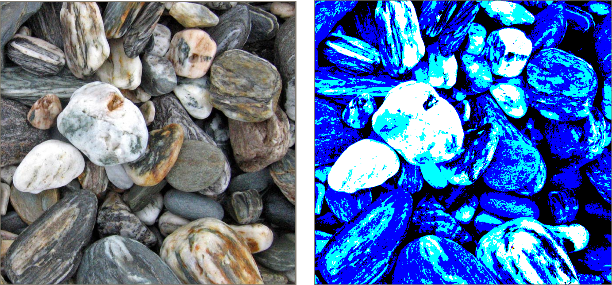
Example Use of an AUMultiField

Here's an example that uses the fields array of an AUMultiField object to do independent thresholding on the three color channels of an image.

void setup() {
 PImage Img = loadImage("07-28-Bruce-Beach-3a.jpg");
 size(Img.width, Img.height);
 image(Img, 0, 0);
 saveFrame("first.tif");
 AUMultiField mf = new AUMultiField(this, 3, width, height);
 mf.RGBfromPixels();
 for (int y=0; y<mf.h; y++) {
   for (int x=0; x<mf.w; x++) {
     float redVal = mf.fields[0].z[y][x];
     float grnVal = mf.fields[1].z[y][x];
     float bluVal = mf.fields[2].z[y][x];
     mf.fields[0].z[y][x] = (redVal > 192) ? 255 : 0;
     mf.fields[1].z[y][x] = (grnVal > 128) ? 255 : 0;
     mf.fields[2].z[y][x] = (bluVal >  64) ? 255 : 0;
   }
 }
 mf.RGBtoPixels(0, 0);
 saveFrame("thresholded.tif");
}

AUCamera

Imaginary Institute Technical Note 7, Fields and Cameras.

When we view a film or video, we are used to seeing small streaks. These may be caused by the motion of the camera, but more often they're the result of fast-moving objects. During the finite time that the cameras physical shutter is open, the image of the moving object on the film or sensor moves, leaving behind a trail. The faster the object moves, the longer and dimmer the trail. After endless hours of movies and videos, most people are unconsciously trained to expect this motion blur, and in fact we often use it as a cue to help us interpret images with fast-moving objects.

Images produced on the computer often represent a frozen instant of time. When we combine them to form an animated sequence (e.g., a video or animated gif), the results can seem to be jerky, or to stutter, or just feel wrong somehow. Often the problem is due to the lack of motion blur, which we expect.

The solution we use here is to produce many images (which I call snapshots) and then the library combines them to produce a final frame, which it then saves to disk. The snapshots are combined as though there was a shutter between the cameras film (or sensor) and its iris. If there are enough snapshots, the results are nicely motion-blurred. As a rule of thumb, start with 4 snapshots per frame, and if your objects are moving too fast and are leaving distinct images, increase the number of snapshots until each frame looks nicely blurred.

The AUCamera object has many options, but the defaults have been chosen so that you'll get very nice results with almost no work. For a more complete and detailed discussion of the AUCamera object, please look at the technical note mentioned above.

One technical point worth noting is that sometimes the frames produced in this manner look darker than the individual snapshots. That's because each snapshot contributes only a small amount of its color to the final image. If your frames are coming out too dark, you can scale them before saving by sending setAutoNormalize(true) to your camera. This option is off by default, because most of the time it's not needed.

Also note that because of the nature of the AUCamera, it's not designed for real-time animations. The AUCamera is for when you're producing frames to later assemble into a movie (or animated gif).

Basic Use

The basic camera scenario requires only three lines of code.

Step 1: Declare a global

Declare a global variable to hold your AUCamera object. don't create the camera yet, though, because the camera builds itself using the graphics windows width and height, and those don't have the right values until your setup() routine creates the graphics window by calling size().

AUCamera MyCamera;

Step 2: Build your camera

After you've called size() in your setup() routine, create the camera itself. The constructor takes four arguments: a pointer to your sketch (using the keyword this), an integer giving the total number of frames in your animation, an integer giving the number of snapshots you'll be generating for each frame, and a boolean telling the camera whether or not to save the frames as they're created (more on this in a moment):

AUCamera(PApplet app, int numFrames, int numExposures, boolean saveFrames);

Here's an example using 5 snapshots per frame, for a movie that's 20 frame long, where we want to save the frames:

MyCamera = new AUCamera(this, 20, 5, true);

Remember, always create your camera after calling size() .

Step 3: Use the camera

To use the camera, just tell it to take an exposure at the end of every draw():

void draw() {
  // draw your picture
 MyCamera.expose();
}

That's all you need to do. Here's what happens by default: the camera will use an open shutter (discussed below), it will create a subfolder named pngFrames in your sketch folder (if it doesn't already exist), and then inside that subfolder, it will store files named frame0000.png, frame0001.png, and so on, each holding one motion-blurred frame. When the camera has saved the number of frames you specified in numFrames, the camera tells Processing to exit, and your program ends.

You can then read your frames into any movie-editing program and assemble them into a movie file, or convert them gif and turn them into an animated gif.

An important extra bit of information that you'll usually get from the camera on each frame is the current time. This is a float that runs from 0, for the first image of your animation, to nearly 1 at the end. The value at the end is just one image's duration short of 1, so that if you loop your animation it will join up seamlessly.

To get the time, just ask the camera for it at the start of your draw() routine:

void draw() {
   float time = MyCamera.getTime();
   // draw your picture
   MyCamera.expose();
}

There are many options you can specify, but one of the most important is which shutter you want to use. So we'll look at shutters next, and then come back to the AUCamera options.

Shutters

The most visible option in the AUCamera object is the shutter. You can use any of several different built-in shutters, and you can even provide your own.

The idea is that every snapshot has an accompanying shutter, which tells the camera how much each pixel of the snapshot contributes to the frame that's being accumulated. You can think of the shutter as a 2D grid of floats. Each pixel has a color (from the snapshot) and a contribution (from the shutter). The color is multiplied by the contribution and the result added into the frame. When the specified number of snapshots have been accumulated, the frame is written to disk, and the film is reset to black, ready for new snapshots.

So if a pixel has a corresponding contribution of 0, it contributes nothing to the accumulating frame. Contributions of 1 mean the pixel makes maximum impact, and values between 0 and 1 scale how much the pixel contributes.

You can overwrite the default shutter by calling shutterType() with the option you prefer (the open shutter is the default):

void setShutterType(int shutterType);

Your choices for shutterType are

• SHUTTER_OPEN
• SHUTTER_UNIFORM
• SHUTTER_BLADE_RIGHT
• SHUTTER_BLADE_LEFT
• SHUTTER_BLADE_DOWN
• SHUTTER_BLADE_UP
• SHUTTER_IRIS

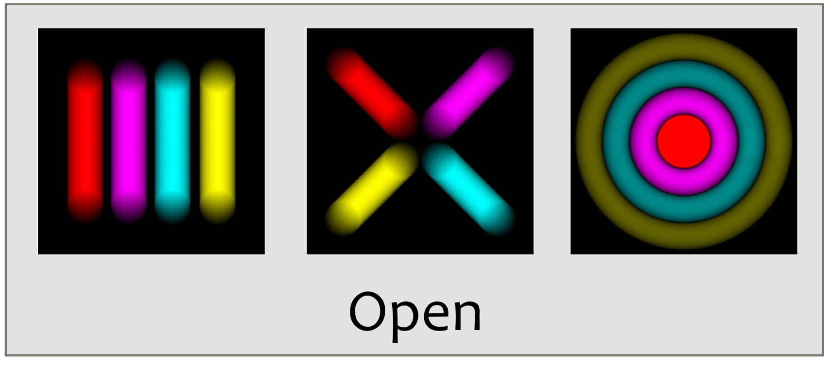
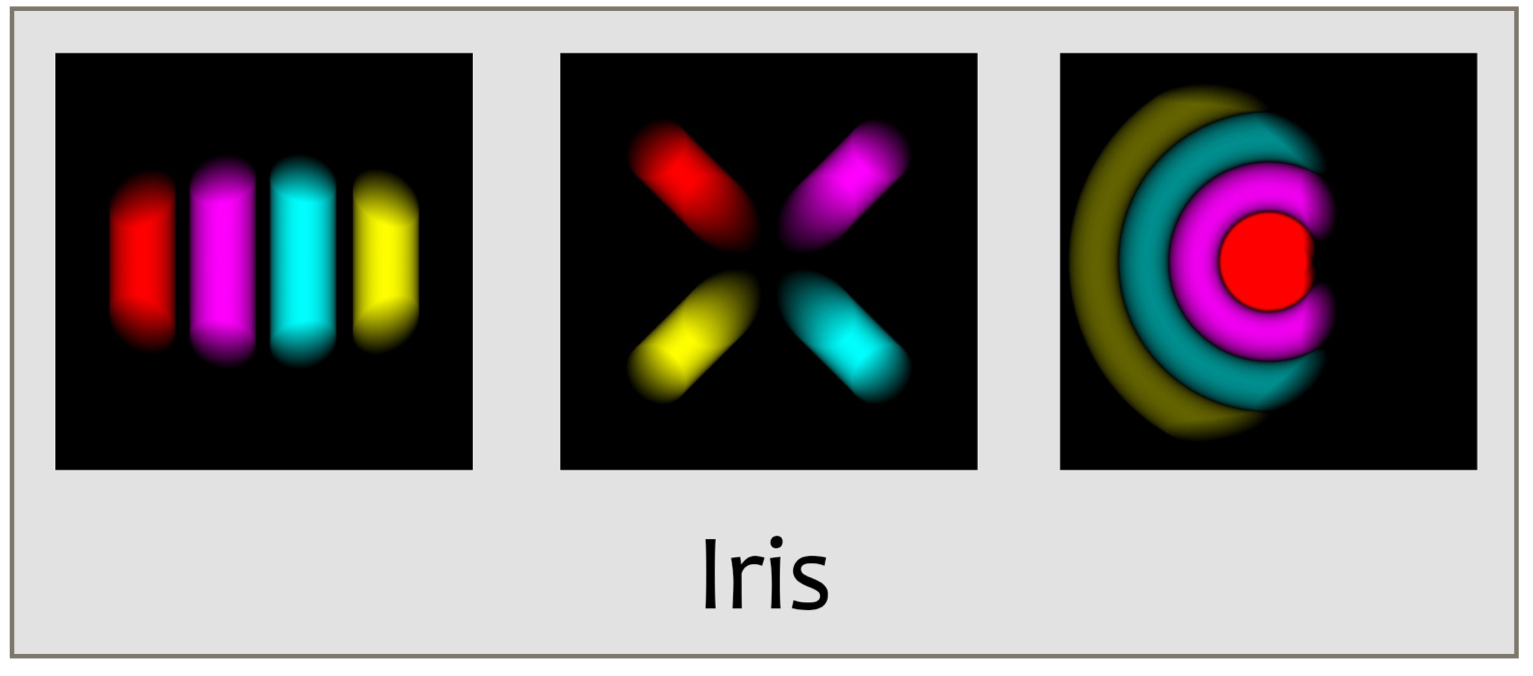
To demonstrate the effect of each shutter, I'll present the results of three different little animations, each involving four circles. The arrows show the motion of the disks in each scene, over the course of a single frame. Note that these motions are enormously exaggerated for the point of illustration. You would probably never have objects moving this far in just one frame.

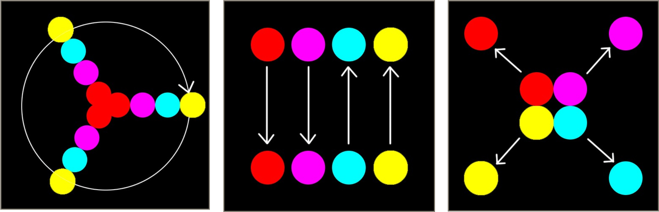
I mentioned above that the longer the motion blur trail, the dimmer it appears, because the object is sending less light to each point on the film. For that reason, the rightmost example (the four balls moving in circles) produces very dim results. For this discussion, I brightened those images up in Photoshop so that you could see whats happening; the other images are untouched. For larger images and more detailed discussion, please consult the tech note mentioned above.

The default shutter is called the open shutter, with type SHUTTER_OPEN, though you can think of it as a non-shutter. In terms of the 2D field of contributions, it is always 1 everywhere. Thus every pixel of every snapshot makes a full contribution to the final frame.

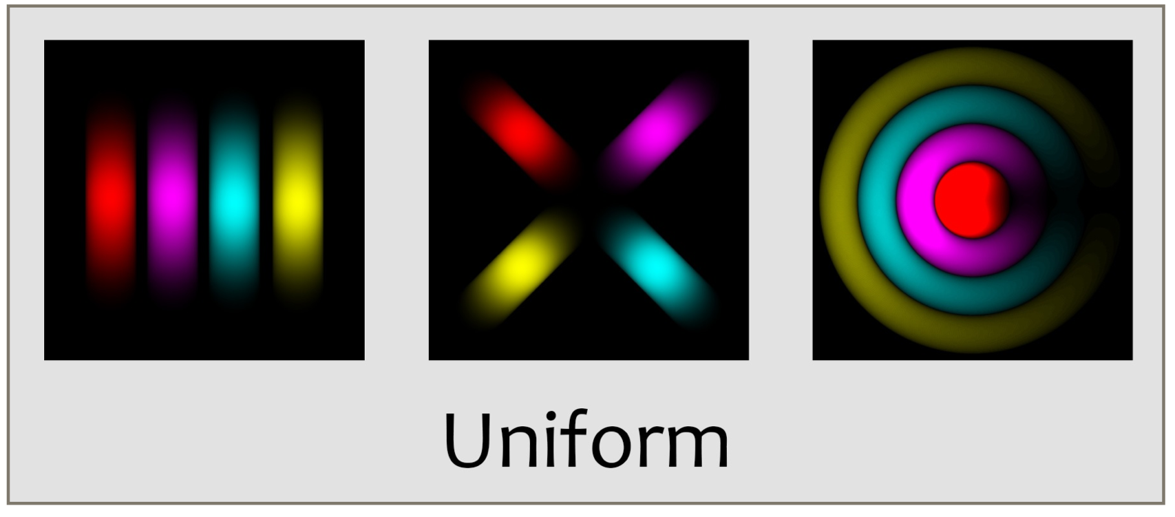
A slightly more sophisticated shutter is the uniform shutter with code SHUTTER_UNIFORM. You can think of this as a sheet of glass placed over the film (or sensor), except that we can control the opacity of the sheet on a moment-to-moment basis. In the camera, this shutter starts out completely opaque, and then the entire sheet becomes increasingly transparent. It stays entirely transparent for a while, and then becomes opaque, reaching total opacity at just the time the final snapshot arrives.

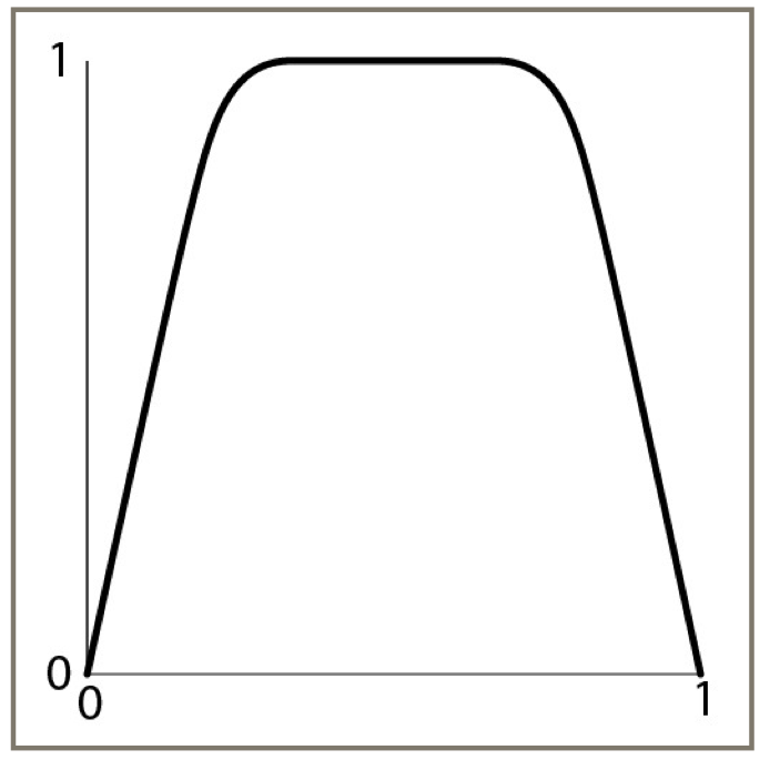
The amount of transparency is controlled by a curve that starts at 0, rises smoothly to 1, and then smoothly drops back down to 0 at the end of the exposure. By default, the rise and fall times take about 25% of the total exposure time, leaving the middle 50% entirely transparent. Here's the default shape of that curve, which controls the one parameter for each moving shutter. You can adjust the shape of this curve using options discussed below.

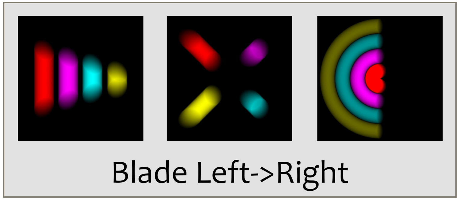
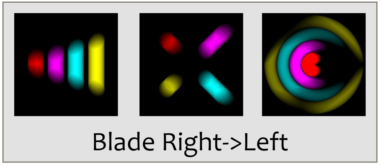
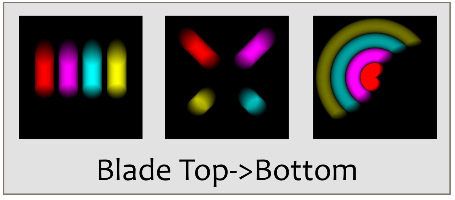
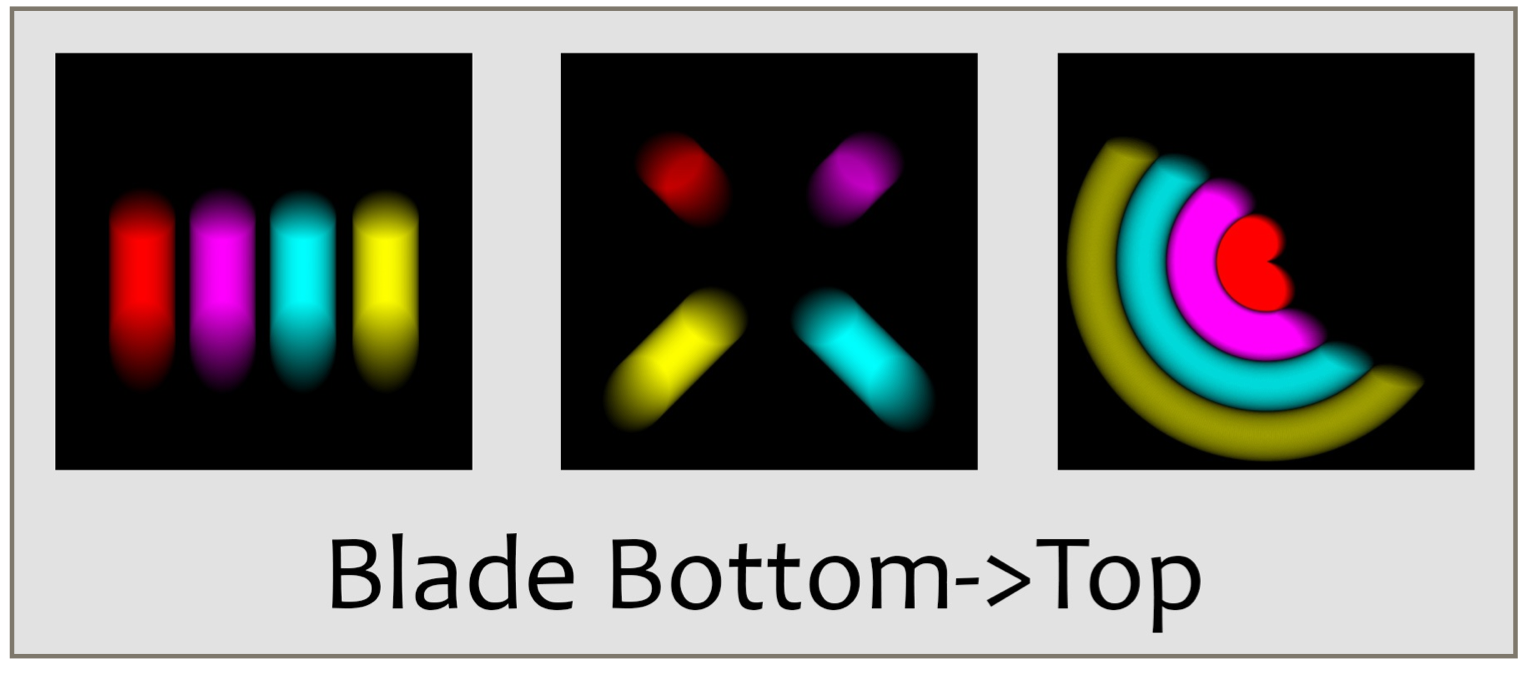
A more physically motivated shutter is the blade shutter, where we imagine that a sheet of opaque material (the blade) is positioned in front of the film. At the start of the exposure, the blade is pulled off to one side, allowing light to strike the film. At the exposuress end, the blade is pushed back into place. The little curve we used for controlling the transparency of the uniform shutter controls the position of the blade. The AUCamera allows you to pull the blade away to the left, right, top, or bottom. Each of the four directions has its own descriptive type: SHUTTER_BLADE_LEFT, SHUTTER_BLADE_RIGHT, SHUTTER_BLADE_DOWN, and SHUTTER_BLADE_UP.

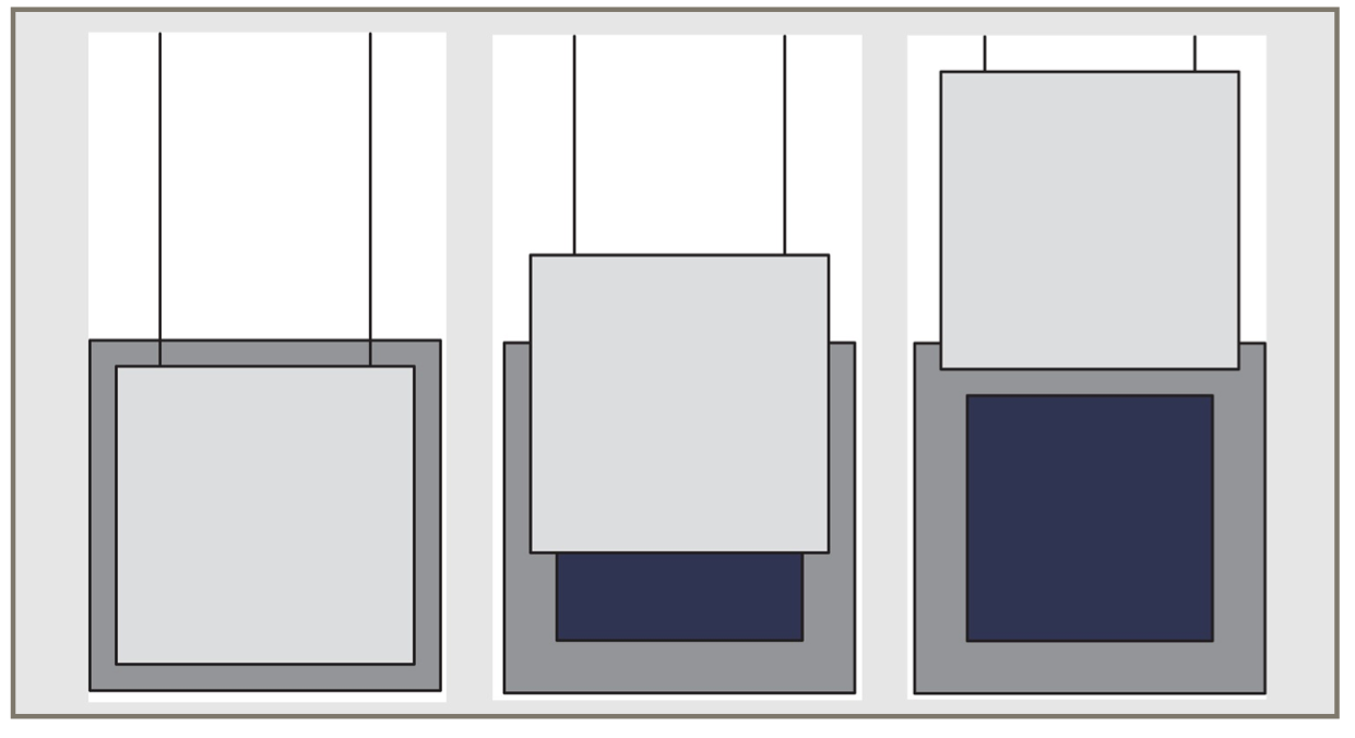
Here's a schematic view of a blade shutter moving upward, or from bottom to top:

Here are the results for the left- and right-moving blades:

Here are the results for the downward- and upward-moving blades.

Finally, an iris shutter of type SHUTTER_IRIS is modeled after a physical device that uses a number of overlapping, triangular metal plates. Each plate is hinged at one vertex, and together they all rotate around their hinges.

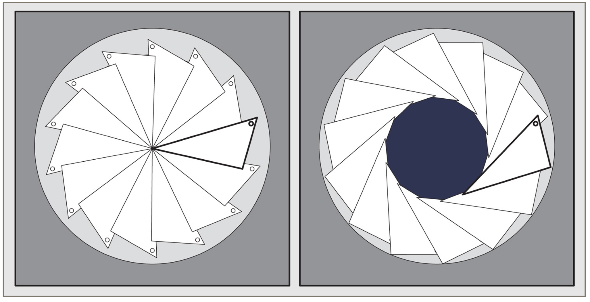
The result is that a near-circle appears in the center of the iris, and eventually grows until the film is completely exposed. As before, at the end of the exposure the shutter closes down again. The size of the opening in the middle of the iris shutter is controlled by the same curve we used above.

The iris shutter is an idealized version of the kind of shutter found in many older film cameras. It had a characteristic sound as the metal plates slid over one another while opening, and a slightly different sound as they closed. The whirring or shushing sound played by many digital cameras and cell phones often sounds to me like a recording of an iris shutter doing its thing. Like a grandfather clock ringing out the hour, it's an anachronistic sound that most people recognize.

Options

You can fine-tune many aspects of the cameras behavior after you've created it.

Set the number of frames to save:

void setNumFrames(int numFrames);

Set the number of exposures in each frame:

void setNumExposures(int numExposures);

Scale each frame to (0,255) using the AUMultiField together method (see AUMultiField section for more details):

void setAutoNormalize(boolean autoNormalize);
(default = false)

Turn off the feature where the camera saves your frames to disk when they're done. You can use this when debugging, but usually the better approach is to get the saveFrames field in your constructor to false. Then when you're done and ready to save, you can just set that back to true.

void setAutoSave(boolean autoSave) 
(default = true)

Set the file format for frames: gif, tif, tga, or jpg (do not include a period). Note that Processing uses Javas library for saving gif files, and that's known to occasionally produce images with visible problems. If you want your frames in gif format, for example to produce an animated gif, I recommend you save them in png, and then use one of the many free utility programs out there to convert your png files to gif.

void setSaveFormat(String saveFormat);
(default = png)

Set the path in your sketch directory where frames are to be saved

void setSavePath(String savePath);
(default = pngFrames)

When you initially create your camera, you might set saveFrames to false while you're developing or debugging your code. This means the camera won't automatically exit when the last frame is collected, and time will just keep rolling on. By default, the value returned by getTime() will wrap from 1 back to 0. If you set timeWrap to false , then the value returned by getTime() will simply increase. Note that this does not affect the value returned by getFrameTime().

void setTimeWrap(boolean timeWrap);

If you want your program to exit when the last frame is saved (default = true)

void setAutoExit(boolean autoExit);

Some animations build on pre-existing images. If you want to generate a bunch of exposures before saving, set this value to the number of exposures you want. These pre-exposures do not have to create full frames.

void setPreRoll(int preRoll);
(default = 0)

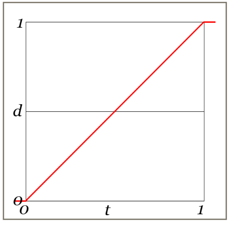
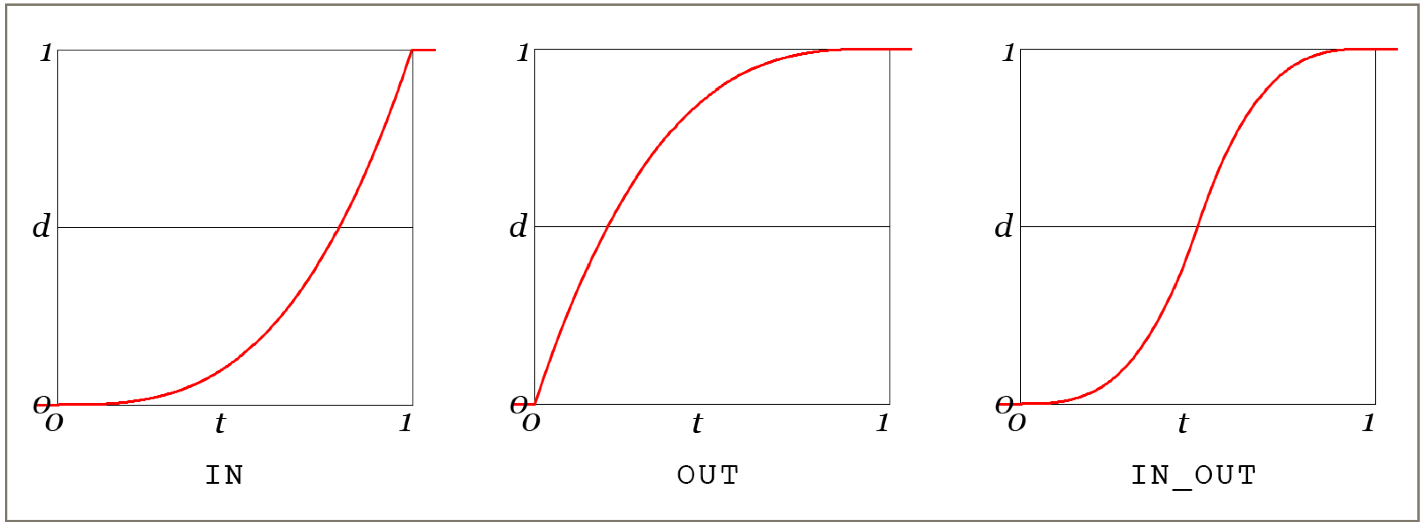
The remaining two options let you shape the curve that controls how the shutters change over time. Generally each shutter has a closed form (where it's blocking the iris completely) and an open form (where the iris is fully exposed). Over the course of a single frame, it goes from closed to open, stays open, then closes again. The speed with which this happens is defined by a symmetrical curve that runs from 0 (at the start of the frame) to 1 (at the end). The value of the curve also runs from 0 to 1.

The ramp time is the fraction from 0 to 1 that identifies where the ramp would end if there was no smoothing. to the right, that's where the red line reaches the value of 1. The blend time is the fraction of the ramp time over which smoothing occurs (note that this is not a fraction of the total exposure, like the ramp time. It's a fraction of the ramp time, from 0 to 1).

The curve controls one parameter for each shutter type. Here's how:

• SHUTTER_OPEN: no effect
• SHUTTER_UNIFORM: opacity (0=opaque, 1=transparent)
• SHUTTER_BLADE_RIGHT: position moving right (0=closed, 1=open)
• SHUTTER_BLADE_LEFT: position moving left
• SHUTTER_BLADE_DOWN: position moving down
• SHUTTER_BLADE_UP: position moving up
• SHUTTER_IRIS: size of circle (0=closed, 1=open)

To set these times, you can use the following two routines after you've created your camera.

void setRampTime(float rampTime);
default = 0.2

void setBlendtime(float blendTime) 
default = 0.25

Getting the Time

Because your draw() routine is just creating images, it's often useful to ask the camera where it is in the frame-making process. You can get this information in two different forms by asking the camera for the current time. In both cases, the time you get back represents the time at the start of the next snapshot. Thus before you've saved any snapshots, the time is 0.

The first form of the time, called simply time, runs from 0 towards 1 over the course of your animation. I say towards 1 because it never quite hits 1. that's because if you're making a cyclic animation, which is very common, you don't want the last frame to be identical to the first, or your animation would have a little stutter at that point.

To get the time, call getTime():

float getTime()

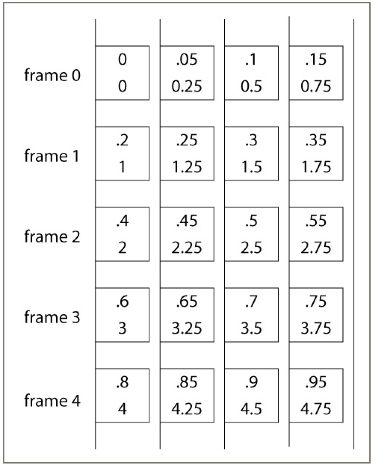
The second form of time, called frame time , gives you a floating-point number, where the integer part tells you which frame your next snapshot will contribute to, and the fractional part identifies how far into that frame the snapshot is located. For example, if you had 5 snapshots per frame, and a frame time of 3.4, you know the next time you call expose() you'll be saving the third snapshot of frame 3 (because with 5 snapshots, they will be at 3.0, 3.2, 3.4, 3.6, and 3.8).

To get the frame time, call getFrameTime() :

float getFrameTime()

In the figure below, each box is a snapshot. The numbers show whats returned by the system before you call expose() for that frame. The upper value is that returned by getTime() , the lower value is whats returned by getFrameTime() .

You can use whichever form of time is most convenient for your animation.

Custom Shutters

You can make your own shutters. The technique is to fill up an AUField with values that indicate how opaque each pixel should be for that exposure. You then hand that field to the camera, which gets the pixels from the screen as usual, but uses your AUField object as the shutter rather than one of the built-in shutters. At each pixel, it finds the corresponding value in your AUField , and it multiplies the pixels RGB values by that number. So to make a shutter opaque at a given pixel, put a value of 0 in the corresponding field entry. To make it transparent, put a value of 1 in there. And of course intermediate values will result in intermediate opacities.

To make an exposure using a custom shutter, call

void exposeWithShutter(AUField customShutter);

If you supply your own shutter, the values of rampTime and bladeTime are ignored. In all other ways, the camera operates as usual.

Suppressing File Output

Each time you call expose(), a number of things happen behind the scenes that keep the AUCamera object running properly. Therefore it's important that you call expose() at the end of every time through draw() , whether you're saving output files or not.

If you're debugging, and you don't want to have to wait to write and save a frame, then set saveFrames to false when you create your camera. This will also set numExposures to 1, which is usually what you want when debugging. If you really want to have multiple exposures per frame when debugging, just follow the constructor with a call to setNumExposures() with the number of exposures per frame you want. When your programs running the way you want, just set saveFrames to true .

Another way to suppress frame writing is to give expose() the argument false :

void expose(false);

This lets you skip saving specific frames, if you need to. Note that if you have multiple exposures per frame (as you usually will), this call will only suppress writing a frame if it's called to create the last exposure for that frame.

Coordinating an AUStepper and an AUCamera

If you're using an AUStepper (see above), the time you get from that objects getFullAlfa() routine will be the same as the cameras getTime() .

If you do want to use an AUStepper in the same sketch as an AUCamera, it's important that they both have the same idea about how long your animation is. Here's a skeleton for keeping things in order:

AUStepper Stepper;
AUCamera Camera;
void setup() {
  int numFrames = 400;   // 400 output frames
  int numExposures = 5;  // 5 snapshots per frame
  float stepLengths = { 3, 5, 2, 5 }; // relative lengths
  int numSnapshots = numFrames * numExposures;   
  Stepper = new AUStepper(numSnapshots, stepLengths);
  Camera = new AUCamera(this, numFrames, numExposures, true);
}

void draw() {
  Stepper.step();  // same result as Camera.getTime();
  switch (Stepper.getStepNum()) {
     case 0: drawStep0(Stepper.getAlfa()); break;
     case 1: drawStep1(Stepper.getAlfa()); break;
  }
  Camera.expose(); // always expose when an image is done!
}

AUCurve, AUBezier, and AUBaseCurve

Imaginary Institute Technical Note 8, Equal Spacing Along Curves.

Curves are useful in graphics programs for lots of reasons. Of course, we can draw them on the screen to create objects. But we can use them to specify the motion path for an object, or describe how a color or a shape (or anything else) changes over time.

Processing supports two kinds of curves: Catmull-Rom (the routines use the word curve) and Bezier (the routines use the word bezier). You make these by giving Processing four points. In addition to drawing the curve, you can get back position information (useful for using the curve as a motion path) by passing the four values and a value for a parameter named t, which runs from 0 at the start to 1 at the end.

This setup is simple and can be useful in many situations. But it has two big drawbacks.

The first problem is that if you ask for points that are equally spaced using the parameter (e.g., t =0.0, .2, .4, .6, .8, 1.0) you will almost never get back equally-spaced points along the curve. that's just how the curve math words.

The second problem is that even if you could space your points evenly along a curve segment, in a big multi-segment curve some of the segments are short and others are long, so if you use the same number of points on all segments theyll be bunched up in the short segments and spread out in the longer ones.

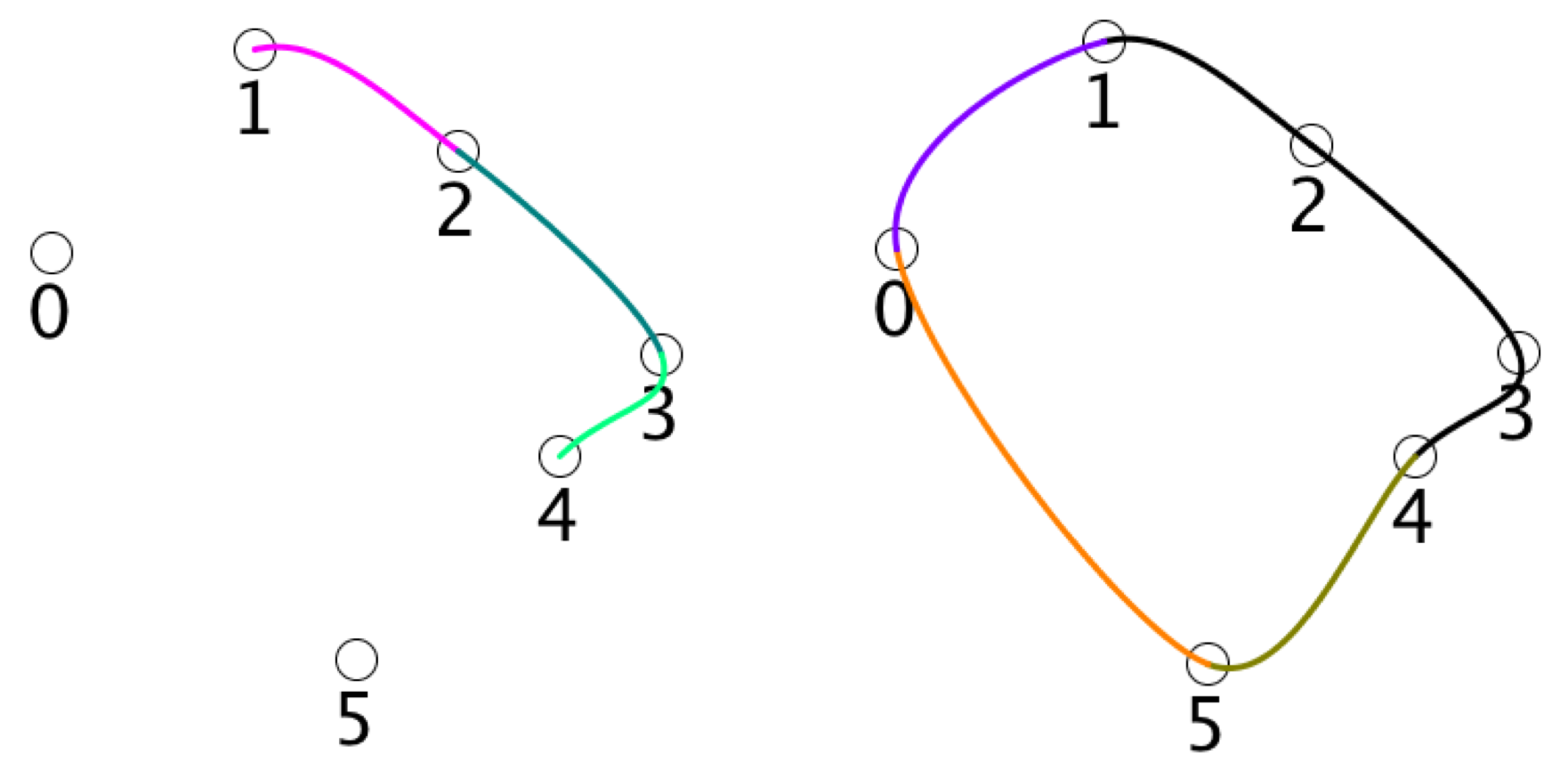
The following picture demonstrates both of these problems. We want 20 points evenly spaced along the entire curve, which is made of five Catmull-Rom segments (they're drawn in different colors). On the left I'm taking 4 samples on each curve at t =0, .25, .5, and .75. You can see that the samples aren't distributed uniformly along any segment, and that they bunch up more tightly in short segments than in long ones. On the right are the points we want.

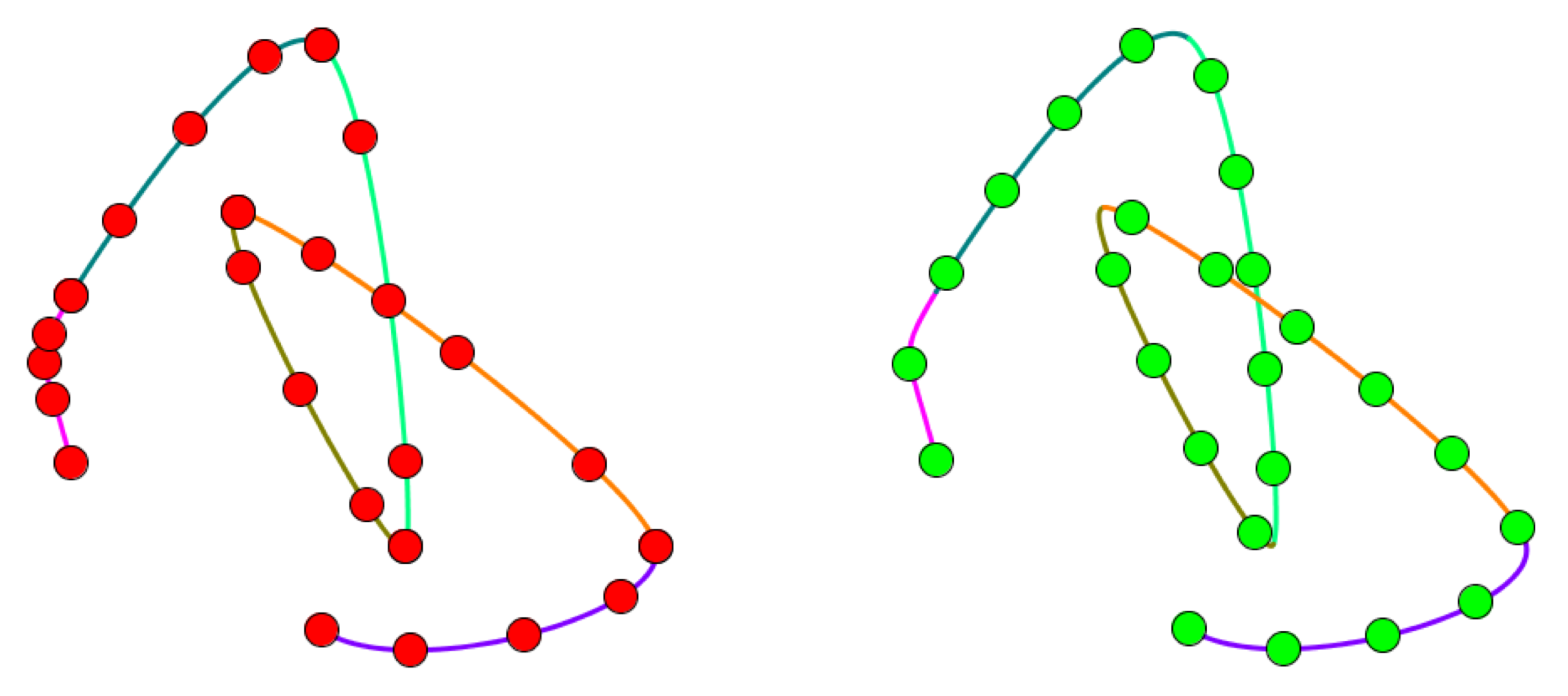
To get the results on the right, create a curve using one of the objects in this section. Then when you ask for a point on the curve, the value of t that you pass in represents a percentage along the curve. As before t =0 is the start of the curve and t =1 is the end, but a value like t =.3 will be 30% of the way along the entire curve, no matter what kind of segments it's made out of.

There are two types of constructors. Create an AUCurve for a Catmull-Rom curve, and an AUBezier for Bezier curves. For each type of curve there are three constructors: shortcuts for single-segment 2D and 3D curves, and more general constructors. Well look at the Catmull-Rom versions first.

AUCurve constructors

AUCurve(float x0, float y0, float x1, float y1, 
        float x2, float y2, float x3, float y3);

AUCurve(float x0, float y0, float z0, 
        float x1, float y1, float z1, 
        float x2, float y2, float z2, 
        float x3, float y3, float z3);

AUCurve(float[][] knots, int numGeomVals, boolean makeClosed);

The first two constructors are conveniences when you're making a curve of only one segment. For multi-segment curve, use the third, more general version.

The third constructor takes three arguments. The first is knots , a 2D array of floats. Each row of the array represents one knot. The geometry information (e.g., x and y values) must come at the start of the row. After that, you can include additional floats, and they will be smoothly interpolated along with the geometry. There must be at least 4 knots your curve.

Because the routines need to distinguish the geometry information from the other floats you might add, the value of numGeomVals tells the constructor how many entries at the start of the row are geometry. For a 2D curve, this would be 2. For a 3D curve, it would be 3. You don't have to stop there: you can have any number of dimensions you like.

Finally, the boolean makeClosed tells the system whether youd like it to close the curve for you, joining it up smoothly and seamlessly. The figure below shows six points that define an open Catmull-Rom curve, and the three new segments the library will make for you if you say you want it to be closed. In a closed curve, all the other data associated with the knots will also form closed, smooth loops. Note that if you close a curve, the point at t =0 is the same as the point at t =1.

AUBezier constructors

Like Catmull-Rom, there are three constructors for Bezier curves. The first two are conveniences for curves of only a single segment. If you're making a bigger curve with multiple segments, use the third, more general version.

AUBezier(float x0, float y0, float x1, float y1, 
         float x2, float y2, float x3, float y3);

AUBezier(float x0, float y0, float z0, 
         float x1, float y1, float z1, 
         float x2, float y2, float z2, 
         float x3, float y3, float z3);

AUBezier(float[][] knots, int numGeomVals, boolean makeClosed);

These constructors follow the same form as the AUCurve versions, so read that discussion to see whats what.

The arguments are all the same, except for the knots array. In a Bezier curve, the first segment requires 4 points. The next section needs only 3 more points, and then 3 more after that, and so on. So the number of knots in your curve must be at least 4, plus any multiple of 3. In other words, n sections require 4+3(n-1) knots.

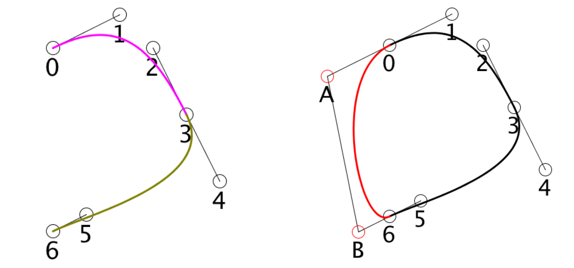
you're responsible for any smoothness you want to create along your curve. A full discussion of Bezier smoothness is beyond the scope of this reference, but remember that the handles around each knot must lie one a line with that knot, at equal distances from it (see points 2, 3, 4 in the picture below).

Closing a Bezier curve requires producing two new handles, labeled A and B in the figure below. This produces one new segment. As with Catmull-Rom curves, in a closed Bezier curve the points t=0 and t=1 are the same. And all other data associated with your knots is also smoothly and seamlessly blended.

Base class AUBaseCurve (no constructors)

Both the AUCurve and AUBezier objects are subclasses of AUBaseCurve.

Though you can't make an AUBaseCurve object yourself, its existence allows you a nice programming convenience.

You can create an array of type AUBaseCurve and then load it up with any mix of AUCurve and AUBeizer objects, in any order. So in one array, you can have a few AUBeizer curves, followed by a few AUCurve curves, and so on.

If you do this, it might be helpful to be able to identify what kind of curve you have when you pick one of the array. To find out, call

int getCurveType();

on each curve you extract from the array. It will return one of these two values:

• CRCURVE
• BEZCURVE

For example:

AUBaseCurve[] myCurves;
// fill up myCurves with a mix of AUCurve and AUBezier objects
for (int i=0; i<myCurves.length; i++) {
   AUBaseCurve curve = myCurves[i];
   // draw CR curves in red, Bezier in green
   switch (curve.getCurveType()) {
      case AUBaseCurve.CRCURVE:  fill(255,0,0); break;
      case AUBaseCurve.BEZCURVE: fill(0,255,0); break;
   }
   // draw the curve
}

Curve methods

Here are the methods that you can use with your curves. Both AUCurve and AUBezier objects respond to these.

To get the X, Y, or Z values of a point at a distance t (remember that this is measured along the entire multi-segment curve), from t=0 at the start to t=1 at the end), call:

float getX(float t);
float getY(float t);
float getZ(float t);

To get one of the other floats attached to your knots, just ask for the value at at that index:

float getIndexValue(float t, int index);

For example, in a 2D curve, the first two entries in each row of knots would be x and then y , so you could retrieve them with getIndexValue(t,0) and getIndexValue(t,1). If you included three more pieces of data after them, you could find their values with:

float myFirstValue = myCurve.getIndexValue(t, 2);
float mySecondValue = myCurve.getIndexValue(t, 3);
float myThirdValue = myCurve.getIndexValue(t, 4);

You can retrieve tangent information in the same way. If you're looking for the geometrical information, use

float getTanX(float t);
float getTanY(float t);
float getTanZ(float t);

and if you want the tangent information for your own data, use

float getIndexTan(float t, int index);

As always, if the curve is closed, the tangents will follow along.

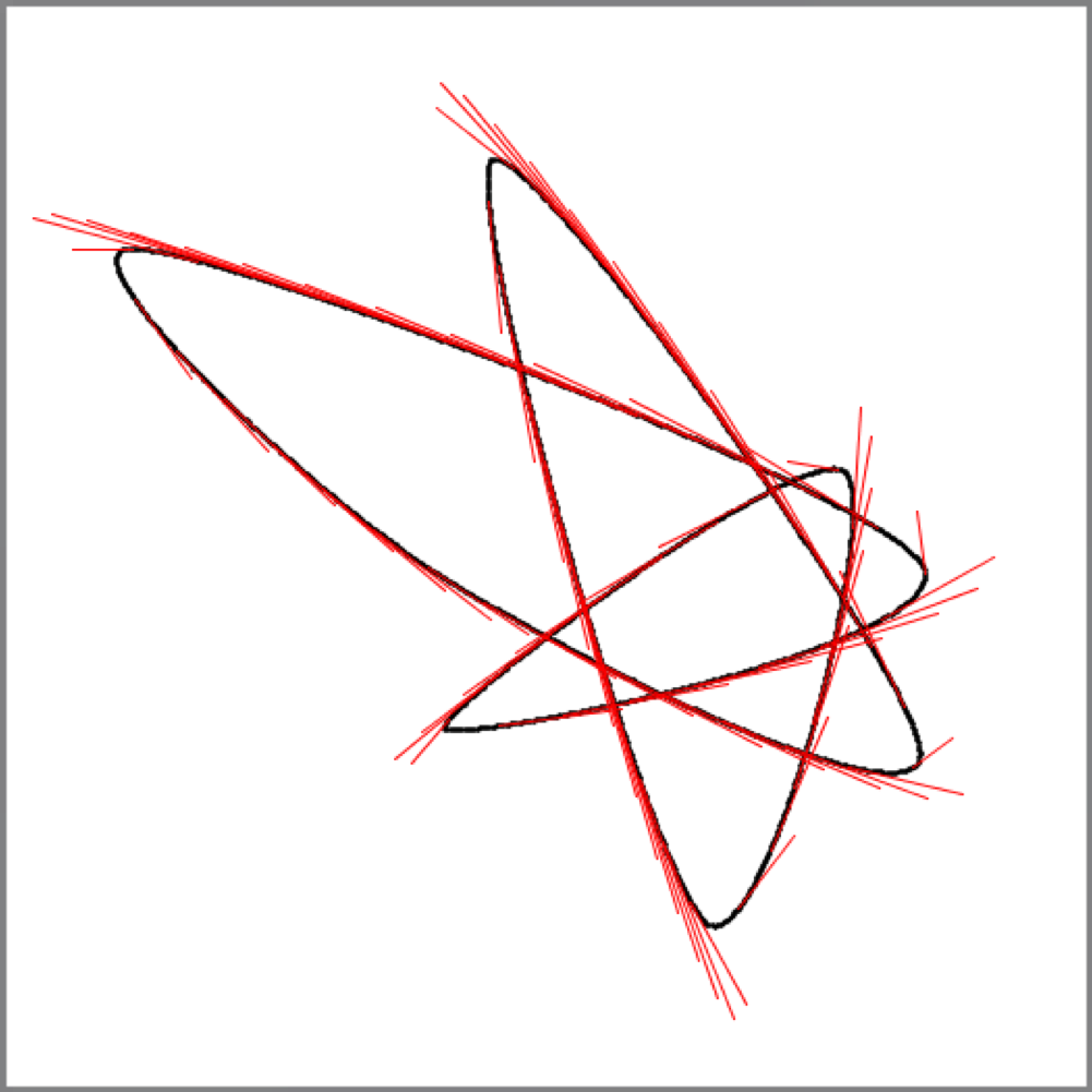
Here is a multi-point AUCurve. with tangents drawn in red.

If your curves change over time, you might want to simply make new ones. If the changes are limited, you might prefer to set the geometry values for a given knot with one of these functions:

void setX(int knotNum, float x);
void setY(int knotNum, float y);
void setZ(int knotNum, float z);

void setXY(int knotNum, float x, float y);
void setXYZ(int knotNum, float x, float y, float z);

To set one of your additional floats, provide the index number and the new value:

void setKnotIndexValue(int knotNum, int index, float value);

You can set a whole row at once. Make sure that the length of the vals array matches the length of the rows of your knots array:

void setKnotValues(int knotNum, float[] vals);

Each time you create a new AUCurve or AUBezier , the system needs to compute some information to make your later requests efficient. If you change any of the values in your knots array using the routines above, that information also gets recomputed. In both cases, that computation takes time. You can make this computation faster (if you don't mind the results becoming less accurate) by reducing the density . You can also make the calculation slower but more precise by increasing the density. This is covered in detail in Imaginary Institute Technical Note 8. The density defaults to 1.0.

To modify the density on a per-curve basis, call

void setDensity(float density);

Normally, using values of t outside the range [0,1] causes the system to let t wrap around. For example, t =1.3 would become merely 0.3, t =187.94 would become 0.94, and so on. If you prefer, you can clamp the values of t so anything less than 0 becomes 0 and anything larger than 1 becomes 1. You control whether to clamp or not on a per-curve basis by calling<

void setClamping(boolean clamp);

Error Messages

I tried to keep error messages to a minimum. For objects, most of the error messages are in the constructors, because I figured that if I let you make an object without objection, it ought to work properly. The functions that you call directly in AULib also do a little bit of checking, for example to make sure that you're not passing in an empty array when that array should hold data.

The error messages are shown in the form

file_name (function_name): message

The messages are deliberately kept very short, but they will alert you that there's a problem, and then you should be able to work things out from there. If you're missing data (for example, passing in an empty array), the library will usually make a very simple replacement for you, so that at least your program will continue to run.

To control whether errors are printed or not, call

void AULib.setErrorLevel(int errorLevel);

where errorLevel can take on these values:

• ERROR_LEVEL_SILENT
• ERROR_LEVEL_NORMAL
• ERROR_LEVEL_QUIT

The first will simply not print out error messages, the second will print them but keep running, and the third will print the error message and then cause your program to exit. This can be useful if your screen is filling up with error messages and you want to see and deal with them one at a time.

For example, to suppress all error messages, call

AULib.setErrorLevel(AULib.ERROR_LEVEL_SILENT);

To reinstate displayed errors, call this again with ERROR_LEVEL_NORMAL.

I'm sure that there are lots of ways to break the library that I haven't checked for or prevented. If you do encounter what you think is a real problem with the library, please let me know (see below for contact information). Sending the shortest program you can write that always triggers the problem is always the best way to help me find and fix the problem for you.

Conclusions

I hope that this library helps you with your work. If you find a bug, please write to me at the address at the top of this document and let me know precisely whats not working properly. The very best way to help me help you is to cut away everything in your program that you can until you're left with the very smallest bit that consistently triggers the problem. Or you could even write a new, very small sketch to trigger the error. Sending me big, complicated programs will usually result in very slow response times. The simpler the program you send, the faster I'll be able to use it myself to find and fix the problem.

Remember that the other Imaginary Institute Technical Notes give you a lot more information on many aspects of library, including more examples and demonstrations. If you're going to use a new section for the first time, I strongly encourage you to take a look at the relevant note! I think it will make things a lot easier and more pleasant.

And don't forget to check out the examples folder provided with the library itself for running code. Getting the most out of any library usually means getting comfortable with the idioms and techniques that match it best, and those examples demonstrate both ideas for each section of the library.

You can always find the latest version of this note, as well as the others mentioned in this document, on the resources page at The Imaginary Institute:

Some other resources related to my work in computer graphics, Processing, and this library:

• My blog: https://www.imaginary-institute.com/blog
• My Twitter feed: @AndrewGlassner
• My home page: http://www.glassner.com

Have fun!