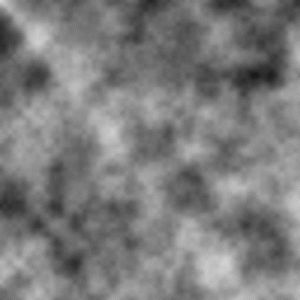
We often use Perlin-esque noise functions to create complex graphics (the noise function built into Processing is just such as function). We can save a value of noise at every pixel in our graphics window, creating a field of noise. The value of these fields is that, unlike white noise, these fields contain visible structure at multiple scales, and that structure usually creates interesting graphics. But when we animate these images they often seem to be missing a certain oomph. This note discusses one way to get that excitement back in there!

To turn a noise-dependent image into an animation, we often take one of two approaches: simply move our objects over an unchanging noise field, or slowly scroll the noise under the graphics window.

But both of these approaches have a very characteristic “look” to them, because the noise field, whether static or moving, reveals itself over time. For example, suppose you have a grid of circles, each of which has a radius based on the value of noise as its center. We’d like the radii to change over time in a noisy way. So if we move the noise, the radii change with it. The result is that the circles don’t seem to be changing in a noisy way. Instead, they look like a fixed pattern is moving under them, which of course is just what is actually happening.

What other choices do we have? One idea is to create a completely new noise field for every frame, but that would destroy any coherence from one frame to the next, causing the images to jump wildly from frame to frame. But what if we make a new field that is only a little different from the one before?

A way to do this is to use multiple noise fields that you blend them over time. In my nomad animation (see previous post), I created four noise fields, simply by filling up the screen with noise four times and saving each one in an AUField object. Then over the course of the animation, each frame began by creating a noise image for that frame. For each pixel, I constructed and sampled a Catmull-Rom spline though the noise values of that pixel. Over the course of the animation, the noise values worked their way through all four fields and back to the first. By overlapping the splines in the usual way for derivative continuity, I got a field that changed smoothly over time. Thus every image was built from its own noise field, but it was a small and smooth change from the field that came before. And since every frame was built from its noise field, and the fields themselves returned to the start, the animation was inherently cyclic.

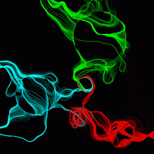
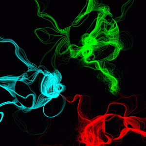
Here are the results. The animation on the left uses just one noise field for the whole animation; things change because the circles (which start the “threads”) are moving. The animation on the right uses exactly the same code, but there are five extra lines that implement the technique above, creating an interpolated noise field at the start of each frame. The single-noise version is nice, but the multiple-noise version has much more energy and dynamic range of motion. (Note: if the images aren’t animating, click on each one to see it in motion).

One noise field

Four noise fields